Rabi oscillations of azimuthons in weakly nonlinear waveguides

Kaichao Jin; Yongdong Li; Feng Li; Milivoj R. Belić; Yanpeng Zhang; Yiqi Zhang

doi:10.1117/1.AP.2.4.046002

Abstract

Rabi oscillation, an interband oscillation, describes periodic motion between two states that belong to different energy levels, in the presence of an oscillatory driving field. In photonics, Rabi oscillations can be mimicked by applying a weak longitudinal periodic modulation to the refractive index. However, the Rabi oscillations of nonlinear states have yet to be introduced. We report the Rabi oscillations of azimuthons—spatially modulated vortex solitons—in weakly nonlinear waveguides with different symmetries. The period of the Rabi oscillations can be determined by applying the coupled mode theory, which largely depends on the modulation strength. Whether the Rabi oscillations between two states can be obtained or not is determined by the spatial symmetry of the azimuthons and the modulating potential. Our results not only deepen the understanding of the Rabi oscillation phenomena, but also provide a new avenue in the study of pattern formation and spatial field manipulation in nonlinear optical systems.

Keywords

azimuthons longitudinally periodic modulation Rabi oscillations weak nonlinearity

1 Introduction

Rabi oscillations were introduced in quantum mechanics,¹ but by now are widely investigated in a variety of optical and photonic systems that include fibers,²^,³ multimode waveguides,⁴^–⁶ coupled waveguides,⁷ waveguide arrays,⁸^–¹⁰ and two-dimensional modal structures.¹¹^,¹² Recently, Rabi oscillations of topological edge states¹³^,¹⁴ and modes in the fractional Schrödinger equation¹⁵ were also reported. Rabi oscillations are interband oscillations that require an AC field to be applied as an external periodic potential. In optics, the longitudinal periodic modulation of the refractive index plays the role of an AC field in temporal quantum systems, and Rabi oscillations are indicated by the resonant mode conversion. As far as we know, the investigation of optical Rabi oscillations thus far has been limited to the linear regime only, and the Rabi oscillation in nonlinear systems is still an open problem that needs to be explored.

The aim of this work is to investigate Rabi oscillations of azimuthons in weakly nonlinear waveguides that is accomplished by applying a weak longitudinally modulated periodic potential. Azimuthons are a special type of spatial soliton; they are azimuthally modulated vortex beams that exhibit steady rotation upon propagation.¹⁶ Generally, azimuthons, especially the ones with higher-order angular momentum structures, are unstable in media with local Kerr or saturable nonlinearities. To overcome the instability drawback, a nonlocal nonlinearity is introduced, and recently published reports demonstrate that the stable propagation of azimuthons can indeed be obtained.¹⁷^–¹⁹ In addition, it was also reported that the spin-orbit-coupled Bose–Einstein condensates can support stable azimuthons as well.²⁰ However, the treatment of nonlocal nonlinearity and spin-orbit-coupled Bose–Einstein condensates is challenging in both theoretical modeling and experimental demonstration. Nevertheless, it has been confirmed that weakly nonlinear waveguides²¹ represent an ideal platform for the investigation of stable azimuthons,²²^,²³ even with higher-order modal structures.

Following this path of inquiry, we first investigate Rabi oscillations of azimuthons in a circular waveguide and then in a square waveguide. Since in this nonlinear three-dimensional wave propagation problem no analytical solutions are known, the mode of inquiry will necessarily be predominantly numerical with some theoretical background. In the circular waveguide, the azimuthons will exhibit Rabi oscillation while rotating during propagation. In the square waveguide, the behavior of the azimuthons is different in two aspects:¹⁵ (i) azimuthons will rotate only if the corresponding Hamiltonian (energy) is bigger than a certain threshold value and (ii) azimuthons will be deformed during propagation. Hence, in this work, we choose azimuthons with large enough energies to avoid wobbling motions in the square waveguide during propagation.

Sign up for Advanced Photonics TOC. Get the latest issue of Advanced Photonics delivered right to you！Sign up now

2 Results

2.1 Theoretical Analysis

The propagation of a light beam in a photonic waveguide can be described by the following Schrödinger-like paraxial wave equation: $i \frac{\partial}{\partial Z} Ψ + \frac{1}{2 k_{0}} (\frac{\partial^{2}}{\partial X^{2}} + \frac{\partial^{2}}{\partial Y^{2}}) Ψ + k_{0} \frac{n_{2}}{n_{b}} {| Ψ |}^{2} Ψ + k_{0} \frac{n (X, Y) - n_{b}}{n_{b}} [1 + μ \cos (δ Z)] Ψ = 0,$ (1)where $Ψ (X, Y, Z)$ is the complex amplitude of the light beam, the quantities $(X, Y)$ and $Z$ are the transverse and longitudinal coordinates, and $k_{0} = 2 π n_{b} / λ_{0}$ is the wavenumber in the medium, where $λ_{0}$ is the wavelength in the vacuum. Other quantities in Eq. (1): $μ ≪ 1$ is the longitudinal modulation strength, $δ$ is the longitudinal modulation frequency, $n_{2}$ is the nonlinear Kerr coefficient, $n (X, Y)$ is the linear refractive index distribution, and $n_{b}$ is the ambient index. In Eq. (1), the refractive index change includes two parts, which are $| n - n_{b} |$ (the linear part) and $n_{2} {| Ψ |}^{2}$ (the nonlinear part). We would like to note that weakly nonlinear waveguides demand not only the linear and nonlinear refractive index changes to be small in comparison with $n_{b}$ , but also the nonlinear part to be much smaller than the linear part. According to the relations $x = X / r_{0}$ , $y = Y / r_{0}$ , $z = Z / (k_{0} r_{0}^{2})$ , $d = k_{0} r_{0}^{2} δ$ , and $σ = sgn (n_{2})$ , with $r_{0}$ being determined by the real beam width, Eq. (1) can be cast into its dimensionless version: $i \frac{\partial}{\partial z} ψ + \frac{1}{2} (\frac{\partial^{2}}{\partial x^{2}} + \frac{\partial^{2}}{\partial y^{2}}) ψ + σ | ψ |^{2} ψ + V [1 + μ \cos (d z)] ψ = 0,$ (2)where $ψ = k_{0} r_{0} \sqrt{| n_{2} | / n_{b}} Ψ$ and $V (x, y) = k_{0}^{2} r_{0}^{2} [n (x, y) - n_{b}] / n_{b}$ . Here we will consider propagation in a deep circular potential $V (x, y) = V_{0} \exp [- {(x^{2} + y^{2})}^{5} / w^{10}]$ , where $w$ characterizes the potential width and $V_{0}$ is the potential depth. Note that it is possible to have a weak nonlinearity even when the potential is deep. Thus the potential can be deep, but the potential modulation can still be shallow. The parameter $σ = 1 (σ = - 1)$ corresponds to the focusing (defocusing) nonlinearity. In this work, we consider the focusing nonlinearity, i.e., we take $σ = 1$ .

Different materials are used to produce waveguides, and silica is one of the most popular, with the typical parameters $n_{b} = 1.4$ , $| n - n_{b} | \leq 9 \times 10^{- 3}$ , and $n_{2} = 3 \times 10^{- 16} {cm}^{2} / W$ for light beams with the wavelengths ranging from the visible to the near-infrared. Without loss of generality, we choose $λ_{0} = 800 nm$ in this work. Therefore, if we choose $V_{0} = 500$ , the value of $r_{0} \approx 25.0 μ m$ is obtained, according to the relation adopted in Eq. (2). Indeed, such a value is reasonable for a multimode fiber.²⁴ According to the wavelength and $r_{0}$ , one learns that the diffraction length is $\sim 7 mm$ . Considering that the group velocity dispersion coefficient is $\sim 35 {fs}^{2} / mm$ at the wavelength of $λ_{0} = 800 nm$ , the dispersion length is on the order of kilometers for a picosecond light beam, which is much longer than the propagation distance taken in this work. As a result, it is safe to neglect temporal effects.

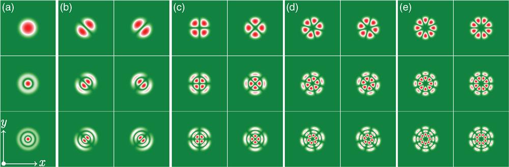
To start with, we consider the modes supported by the deep potential alone; therefore, the nonlinear term and the longitudinal modulation in Eq. (2) are initially neglected. The corresponding solution of the reduced linear Eq. (2) can be written as $ψ (x, y, z) = u (x, y) \exp (i β z)$ , where $u (x, y)$ is the stationary profile of the mode and $β$ is the propagation constant. Plugging this solution into the reduced Eq. (2), one obtains $β u = \frac{1}{2} (\frac{\partial^{2}}{\partial x^{2}} + \frac{\partial^{2}}{\partial y^{2}}) u + V u,$ (3)which is the linear steady-state eigenvalue problem of Eq. (2) when $σ$ and $μ$ are set to zero. Equation (3) can be solved by utilizing the plane-wave expansion method, and the eigenstates supported by the deep potential $V (x, y)$ can be easily obtained. In Fig. 1, the first-order as well as higher-order basic modes, degenerate dipole modes, degenerate quadrupole modes, degenerate hexapole modes, and degenerate octopole modes that can exist in the potential are displayed. Here the term “degenerate” means that all modes feature the same propagation constants, in the usual optical meaning. These linear modes will be used as the input modes of the more general nonlinear and modulated modes of the complete Eq. (3).

Figure 1.(a) Basic modes, (b) degenerate dipole modes, (c) degenerate quadrupole modes, (d) degenerate hexapole modes, and (e) degenerate octopole modes. First row: first-order modes, second row: second-order modes, and third row: third-order modes. The panels are shown in the window $- 2 \leq x \leq 2$ and $- 2 \leq y \leq 2$ . Other parameters: $V_{0} = 500$ and $w = 1$ .

Therefore, to seek approximate azimuthons in weakly nonlinear waveguides, one takes the degenerate modes and makes a superposition of them as the initial wave $ψ (x, y) = A [u_{1} (x, y) + i B u_{2} (x, y)] \exp (i β z),$ (4)where $A$ is an amplitude factor, $1 - B$ is the azimuthal modulation depth, and $u_{1, 2} (x, y)$ are the degenerate linear modes (see examples in Fig. 1). Thus we set the transverse profile of the azimuthon at the initial place as $U (x, y, z = 0) = A [u_{1} (x, y) + i B u_{2} (x, y)]$ (5)and numerically propagate it to obtain an output mode at an arbitrary $z$ . We should note that the inputs depicted by Eq. (5) do not rotate in a linear medium, since the modes are degenerate. Rotation appears only when the nonlinearity is added to the model.

In Fig. 2, we display such approximate azimuthons with $A = 0.4$ and $B = 0.5$ . One finds that the phase of azimuthons is nontrivial, displaying angular momentum and topological charge. For dipole azimuthons the topological charge is $\pm 1$ , whereas for quadrupole, hexapole, and octopole azimuthons the values are $\pm 2$ , $\pm 3$ , and $\pm 4$ , respectively. As expected, these azimuthons will rotate with a constant angular frequency $ω$ during propagation when the nonlinear term in Eq. (2) is included. Therefore, the wave $U (x, y, z)$ can be rewritten as $U (r, θ - ω z)$ in polar coordinates, where $r = \sqrt{x^{2} + y^{2}}$ and $θ$ is the azimuthal angle in the transverse plane $(x, y)$ . This fact allows for a bit of theoretical analysis.

Figure 2.Amplitude and phase of (a)–(d) the first-order and (e)–(h) the second-order azimuthons constructed from (a) and (e) the degenerate dipoles, (b) and (f) the quadrupoles, (c) and (g) the hexapoles, and (d) and (h) the octopoles. The panels are shown in the window $- 2 \leq x \leq 2$ and $- 2 \leq y \leq 2$ . Other parameters: $A = 0.4$ and $B = 0.5$ .

After plugging Eq. (4) into Eq. (2) with $μ = 0$ , multiplying by $U^{*}$ and $\partial_{θ} U^{*}$ , respectively, and integrating over the transverse coordinates, one ends up with a linear system of equations: $- β P + ω L_{z} + I + N = 0, - β L_{z} + ω P^{'} + I^{'} + N^{'} = 0,$ (6)where $P = \iint {| U |}^{2} d x d y$ , $L_{z} = - i \iint (- y \partial_{x} U + x \partial_{y} U) U^{*} d x d y$ , $P^{'} = \iint {| - y \partial_{x} U + x \partial_{y} U |}^{2} d x d y$ , $I = \iint U^{*} Δ_{⊥} U d x d y$ , $N = \iint (σ {| U |}^{2} + V) {| U |}^{2} d x d y$ , $I^{'} = i \iint (- y \partial_{x} U^{*} + \partial_{y} U^{*}) Δ_{⊥} U d x d y$ , and $N^{'} = i \iint (σ {| U |}^{2} + V) (- y \partial_{x} U^{*} + x \partial_{y} U^{*}) U d x d y$ . Obviously, the quantities $P$ and $L_{z}$ stand for the power and angular momentum of the beam, and $P^{'}$ is the norm of the state $\partial_{θ} U$ . The integrals $I$ and $I^{'}$ are related to the diffraction mechanism of the system, whereas $N$ and $N^{'}$ account for the waveguide and nonlinearity. The angular frequency of the azimuthon during propagation can be obtained by directly solving Eq. (6), that is $ω = \frac{P (I^{'} + N^{'}) - L_{z} (I + N)}{L_{z}^{2} - P P^{'}} .$ (7)

After these preliminaries, we are ready to address the Rabi oscillation of azimuthons. To this end, we adopt the superposition of two azimuthons $U_{m, n} (x, y) \exp (i β_{m, n} z)$ as an input $ψ = c_{m} (z) U_{m} (x, y) \exp (i β_{m} z) + c_{n} (z) U_{n} (x, y) \exp (i β_{n} z),$ (8)where $c_{m, n} (z)$ are the slowly varying complex amplitudes of the azimuthons and the modulation frequency is $d = β_{m} - β_{n}$ . Plugging Eq. (8) into Eq. (2), and without considering the nonlinear term [but still on the level of analysis of Eq. (3)], one obtains $i \frac{\partial c_{m}}{\partial z} U_{m} \exp (i d z) + \frac{1}{2} μ c_{m} V U_{m} [1 + \exp (2 i d z)] + i \frac{\partial c_{n}}{\partial z} U_{n} + \frac{1}{2} μ c_{n} V U_{n} [\exp (i d z) + \exp (- i d z)] = 0 .$ (9)

Since the azimuthons are constructed based on Eq. (5), they satisfy the relation $⟨ U_{m}, U_{n} ⟩ \neq 0$ if $m = n$ and $⟨ U_{m}, U_{n} ⟩ = 0$ if $m \neq n$ , thus forming a complete set of eigenstates. Here we borrowed the bra-ket notation from quantum mechanics. Note that the orthogonality of azimuthon shapes is only valid in the weakly nonlinear regime. As a result, one obtains two coupled equations based on Eq. (9): $i \frac{\partial c_{m}}{\partial z} + \frac{1}{2} μ \frac{⟨ U_{m} V U_{n} ⟩}{⟨ U_{m} U_{m} ⟩} c_{n} = 0, i \frac{\partial c_{n}}{\partial z} + \frac{1}{2} μ \frac{⟨ U_{n} V U_{m} ⟩}{⟨ U_{n} U_{n} ⟩} c_{m} = 0,$ (10)where $⟨ U_{m} V U_{n} ⟩ = \iint r U_{m}^{*} V U_{n} d r d θ$ , with the asterisk representing the conjugate operation. Based on Eq. (10), the period of the Rabi oscillation can be obtained as $z_{R} = \frac{π}{| Ω_{R} |},$ (11)where $Ω_{R} = \frac{μ}{2} \frac{⟨ U_{m} V U_{n} ⟩}{\sqrt{⟨ U_{m} U_{m} ⟩ ⟨ U_{n} U_{n} ⟩}} .$ (12)

We note that the azimuthon conversion happens at half of the period, i.e., at $z_{R} / 2$ . Note also that the Rabi spatial frequency directly depends on the modulation strength $μ$ .

2.2 Circular Waveguide

We investigate the propagation of azimuthons in the circular weakly nonlinear waveguide by including the longitudinal modulation, and the results are displayed in Fig. 3. Without loss of generality, we choose the dipole and hexapole azimuthons, which are shown in Figs. 3(a) and 3(b), respectively. By taking the dipole azimuthon as an example ^[Fig. 3(a)], we want to see whether the Rabi oscillation between the dipole azimuthon ^[Fig. 2(a)] and its corresponding second-order dipole azimuthon ^[Fig. 2(e)] can be established. So, to induce resonance, we set the modulation frequency to be the difference between the eigenvalues of the two modes, which is $d \approx 25.2$ . As shown by Eq. (12), the period of the Rabi oscillation is expected to depend on the modulation strength $μ$ , and here we set it to be $μ \approx 0.031$ to make the period $z_{R} \sim 60$ . As a consequence, one expects to see the second-order dipole azimuthon at a distance $\sim 30$ after turning on the longitudinal modulation.

Figure 3.Rabi transition of (a) a dipole and (b) a hexapole. In each case, the propagation is shown by the isosurface plot above which amplitude distributions at selected distances are shown. In both cases, the weak longitudinally periodic modulation exists in the region $30 \leq z \leq 90$ , with $d \approx 25.2$ and $μ \approx 0.031$ in (a) and $d \approx 36.36$ and $μ \approx 0.014$ in (b). (c) The Rabi oscillation period $z_{R}$ versus the frequency detuning $ℓ$ .

In Fig. 3(a), the propagation of the dipole azimuthon is exhibited as a three-dimensional (3-D) isosurface plot, in which the longitudinal modulation exists only in the interval $30 \leq z \leq 90$ . When the propagation distance is smaller than $z \leq 30$ , one in fact observes the stable rotational propagation of the dipole azimuthon. The selected amplitude distributions at $z = 0$ and $z = 30$ are shown above the 3-D isosurface plots. In the interval $30 \leq z \leq 90$ , which is about one period of the Rabi oscillation, the oscillation between the dipole azimuthon and the second-order azimuthon is displayed, in which the dipole azimuthon completely switches to the second-order azimuthon at $z = 60$ . Indeed, the corresponding amplitude distribution is the same as that in Fig. 2(e) except for rotation, and the reason is quite obvious—azimuthons rotate steadily during propagation. When the propagation distance reaches $z = 90$ , the dipole azimuthon is recovered and the longitudinal modulation is also lifted at the same time. Therefore, one observes a stable rotating dipole azimuthon in the interval $90 \leq z \leq 120$ and the amplitude distributions at $z = 90$ and $z = 120$ , which are dipole azimuthons explicitly, and are shown above the isosurface plot. The analogous propagation dynamics of the hexapole azimuthon is shown in Fig. 3(b), the setup of which is the same as that of Fig. 3(a); it also clearly displays the Rabi oscillation of a higher-order azimuthon.

Here we would like to note that the Rabi oscillation is not feasible between two arbitrary azimuthons. Only azimuthons with similar structures (e.g., the dipole and the higher-order dipole azimuthons) can switch between each other, and azimuthons with different symmetries (e.g., the dipole and the quadrupole azimuthons) will not, because the overlap integrals in general are zero, $⟨ U_{m} V U_{n} ⟩ = 0$ . Note also that the Rabi oscillation between two modes with opposite symmetry is also possible if the potential is antisymmetrically modulated in the transverse plane.²⁵

Generally, there must exist some frequency detuning $ℓ = d - d^{'}$ between the real modulation frequency $d^{'}$ and the resonant frequency $d$ . Therefore, it is reasonable to have a look at the efficiency of the azimuthon conversion versus the detuning $ℓ$ . Unfortunately, one cannot obtain a direct measure of the efficiency via the projection of the field amplitude $ψ$ on the targeting azimuthons due to the rotation of azimuthons during propagation. However, the efficiency is reflected on the Rabi oscillation period $z_{R}$ —the bigger the value of $z_{R}$ , the bigger the efficiency.¹³^–¹⁵ The dependence of $z_{R}$ on the frequency detuning $ℓ$ is shown in Fig. 3(c). As expected, one finds that the efficiency of azimuthon conversion is the biggest at the resonant frequency, and it reduces with the growth of the frequency detuning $ℓ$ .

2.3 Square Waveguide

Now we investigate the azimuthon transition in a square waveguide, which is generated by the potential in Eq. (2) in the form $V (x, y) = V_{0} \exp [- (x^{10} + y^{10}) / w^{10}]$ . Again, we solve for the linear eigenmodes supported by the deep square waveguide using the plane-wave expansion method. Connected with the geometry of the potential, the amplitude distributions of the linear modes are more complex than those in the regular circular waveguide; therefore, we denote them as the deformed modes. In Fig. 4, we display three kinds of deformed modes and the corresponding azimuthons, which will transform mutually because of the relation $⟨ U_{m} V U_{n} ⟩ \neq 0$ .

Figure 4.(a) Rabi transition of a deformed dipole. (b) The amplitude and phase of the azimuthon based on the dipole in (a). (c) The transition of a deformed hexapole. (d) The amplitude and phase of the azimuthon based on the hexapole in (c). (e) The transition of a deformed higher-order dipole. (f) The amplitude and phase of the azimuthon based on the higher-order dipole in (e). The panels are shown in the window $- 2 \leq x \leq 2$ and $- 2 \leq y \leq 2$ . Other parameters: $A = 0.4$ and $B = 0.5$ .

Different from the azimuthons in circular waveguides, the azimuthons in square waveguides rotate conditionally. Due to the symmetry of the square waveguide, a rotating azimuthon will deform, i.e., its profile will change. Without considering nonlinearity, the linear superposition of two degenerate modes [e.g., dipoles in Fig. 4(a), labeled as $u_{1, 2} (x, y)$ ] is also a dipole solution in the square potential, as $u_{1, 2}^{'} (x, y) = [u_{1} (x, y) \pm u_{2} (x, y)] / \sqrt{\iint {| u_{1} (x, y) \pm u_{2} (x, y) |}^{2} d x d y}$ . We found that an azimuthon in a square waveguide will rotate when the condition $H (ψ) > H (u_{1, 2}^{'})$ is met. Here $H$ represents the Hamiltonian of the model.²² Even though the wobbling azimuthons can be established in our numerical simulations, we are more interested in the rotating azimuthons, so we set again $A = 0.4$ and $B = 0.5$ in this section to guarantee the rotation of azimuthons during propagation.

Thus the azimuthons will be deformed during propagation because of the symmetry of the potential, hence to exhibit the azimuthon conversion in a more clear way one has to properly choose the value of $μ$ to make the Rabi oscillation period almost equal to one half of the target azimuthon rotation period, since the modulation frequency $d$ is determined beforehand. Numerical simulations reveal that the rotation periods of the hexapole azimuthon and the higher-order dipole azimuthon are $\sim 148.4$ and $\sim 146.4$ , respectively. Therefore, according to Eq. (12), the modulation strength $μ$ for the two cases should be $\sim 0.085$ and $\sim 0.034$ , respectively. The numerical demonstration of the Rabi oscillation is shown in Fig. 5. Different from the setting for the case of a circular waveguide, the longitudinal modulation always accompanies the square waveguide.

Figure 5.(a) Transition between dipole and hexapole azimuthons with $d \approx 25.2$ and $μ \approx 0.085$ . (b) Transition between dipole and hexapole azimuthons with $d \approx 22.1$ and $μ \approx 0.034$ . The weak longitudinally periodic modulation has to always exist during propagation.

As shown in Fig. 5(a), the hexapole azimuthon is obtained at $z \sim 37.1$ (one half of the Rabi oscillation period and also a quarter of the rotation period of the hexapole azimuthon), whereas in Fig. 5(b) the higher-order dipole azimuthon is obtained at $z \sim 36.6$ . When the propagation distance reaches one Rabi oscillation period, the dipole azimuthon is recovered with a small deformation. To show the azimuthon conversion more transparently, we also display the corresponding phase distributions. Evidently, there is only one phase singularity in the phase of the dipole azimuthon (the topological charge is 1), five singularities for the hexapole azimuthon (the topological charge is 3), and nine for the higher-order dipole azimuthon (the topological charge is again 1). As seen, the phase distributions are in accordance with the expectations and with those displayed in Fig. 4.

3 Conclusion

We investigated and demonstrated Rabi oscillations of azimuthons in weakly nonlinear waveguides with weak longitudinally periodic modulations. Based on the coupled mode theory, we find the period of Rabi oscillation, which is affected by the modulation strength and also by the spatial symmetry of azimuthons. The analysis is feasible for both circular and square waveguides and can be extended to the waveguides of other symmetries.

Based on the model considered in this work, the switching between a vortex-carrying azimuthon and a multipole that is free-of-vortex will not happen. The reason is that the initial azimuthon is composed of two degenerate modes $u_{1, 2}$ that will switch into another two degenerate modes $u_{3, 4}$ during propagation. So the output is a composition of $u_{3, 4}$ , which also carries a vortex. However, if the potential is modulated transversely in a proper manner, such a switch becomes possible once both the longitudinal and transverse phase matching is satisfied.