
Yun Cao, Jichuan Xiong, Xuefeng Liu, Zhiying Xia, Weize Wang, N. P. Yadav, Weiping Liu. Sensing of ultrasonic fields based on polarization parametric indirect microscopic imaging[J]. Chinese Optics Letters, 2019, 17(4): 041702
- Chinese Optics Letters
- Vol. 17, Issue 4, 041702 (2019)
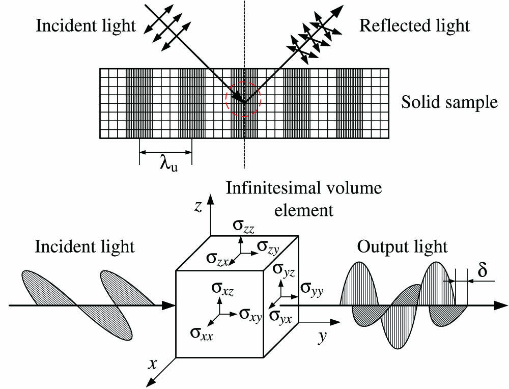
Fig. 1. Schematic diagram of a change in polarization status of light through a solid sample in which an ultrasonic wave propagates. Under the influence of the ultrasonic wave (wavelength
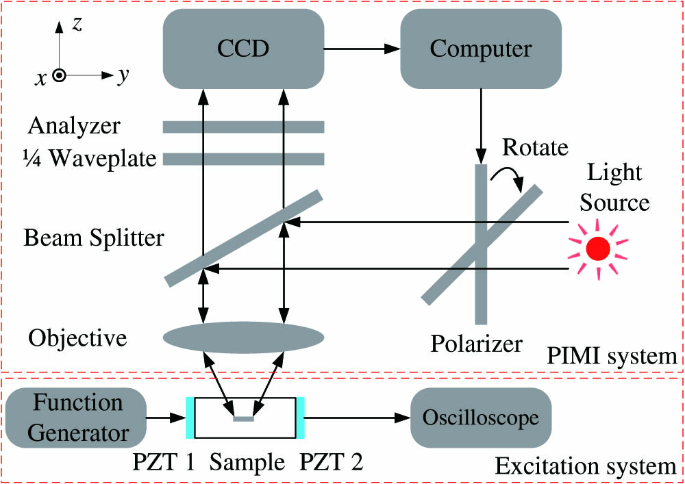
Fig. 2. Experimental setup of ultrasonic field sensing. It consists of an ultrasonic excitation system and a PIMI system. The excitation system was employed to generate ultrasonic waves in the sample, and the PIMI system was used to image and characterize the ultrasonic field by extracting variations of optical properties of the sample with and without ultrasonic excitation.
Fig. 3. PIMI images under different ultrasonic conditions (a)–(c) without and (d)–(f) with ultrasonic excitation. (a) and (d) Average of polarization intensities
Fig. 4. PIMI images of the Stokes parameters under different ultrasonic conditions (a)–(d) without and (e)–(h) with ultrasonic excitation. (a), (e)
Fig. 5. Difference between PIMI images without ultrasonic excitation and those with ultrasonic excitation. (a)
Fig. 6. Image of 3(c) , (e) difference between (b) and Fig. 3(c) , (f) extracted intensity curves along the line in (d) and (e).
Fig. 7. PIMI images under different ultrasonic conditions (a)–(c) without and (d)–(f) with ultrasonic excitation: (a) and (d)

Set citation alerts for the article
Please enter your email address
© Copyright 2018-2021 | Chinese Laser Press. All Rights Reserved 沪ICP备15018463号-20