Sensing of ultrasonic fields based on polarization parametric indirect microscopic imaging

Yun Cao; Jichuan Xiong; Xuefeng Liu; Zhiying Xia; Weize Wang; N. P. Yadav; Weiping Liu

doi:10.3788/COL201917.041702

Abstract

This Letter tackles the issue of non-contact detection of ultrasonic fields by utilizing a novel optical method based on the parametric indirect microscopic imaging (PIMI) technique. A general theoretical model describing the three-dimensional anisotropic photoelastic effect in solid was developed. The mechanism of polarization status variations of light passing through the stress and strain fields was analyzed. Non-contact measurements of the ultrasonic field propagating in an isotropic quartz glass have been fulfilled by the PIMI technique under different ultrasonic excitation conditions. PIMI parameters such as

\sin δ

, Φ, and the Stokes parameters have been found to be sensitive to ultrasonic fields.

Inspection techniques based on ultrasonic waves were widely used in various applications, such as crack detection in industrial parts, medical ultrasound diagnosis, and the recently emerged photoacoustic imaging technology for biomedical tissues, due to strong penetration, good direction, and non-dangerous nature of ultrasonic waves^[1–3]. One of the essential elements of inspection techniques based on ultrasonic waves is the method for effective detection of ultrasonic waves in different kinds of materials, which can be categorized into two groups according to their ways of operation, i.e., contact and non-contact ultrasonic detection methods. Contact ultrasonic detection methods usually use contact transducers made of piezoelectric materials to generate and detect ultrasonic waves^[4,5]. Although various kinds of ultrasonic transducers have been developed and become commercially available, techniques adopting these transducers are generally restricted in contact measurement and detection bandwidth, which leads to limitations of their spatial resolution.

As a consequence, more and more attention has been paid to the non-contact ultrasonic detection methods that enable fast scanning and remote measurement to overcome the difficulty of contact measurement, which include electrical and optical methods. Electrical non-contact transducers, such as a capacitance micromachined ultrasonic transducer (CMUT)^[6,7], electromagnetic acoustic transducer (EMAT)^[8], and air-coupled ultrasonic transducer (ACUT)^[9], need to be placed at a short distance from the surface of the sample to detect ultrasonic waves. Although they have several advantages over the traditional piezoelectric transducer, they are limited by their short operation distance and low efficiency for many applications. Optical methods, including interferometric methods such as the Mach–Zehnder interferometer^[10,11], full-field speckle interferometry^[12], the low-coherence interferometer^[13], the Fabry–Perot polymer film sensor^[14], the polymer micro-ring resonator^[15–17], and the surface plasmon resonance detector^[18], and non-interference methods, such as optical reflection^[19,20], diffraction^[21], and deflection techniques^[22], have been developed and applied to a wide range of applications. They demonstrated great potential and promising prospects for ultrasonic and photoacoustic imaging and sensing due to their high sensitivity, superior wide bandwidths, small effective active sizes, as well as other merits. Towards the full-field imaging of ultrasonic fields, many efforts have been made based on the above detection principles, and various visualization techniques were developed and some commercialized, including phase detection techniques^[10,11,23], the Schlieren technique^[24], shadowgraphy^[25,26], scanning laser Doppler vibrometry^[27], and the photoelastic technique^[28,29]. However, the Schlieren and photoelastic techniques were attractive in visualizing the ultrasonic field in a transparent medium. Shadowgraphy was often used for visualization of a shockwave or very high-pressure fields due to its low sensitivity. The scanning laser Doppler vibrometry has limitations on measurement speed. An optical technique that can rapidly visualize ultrasonic fields with high spatial resolution and require minimal post-processing of data is still attractive.

In this Letter, we proposed a polarization microscopic imaging technique for ultrasonic field sensing based on the reported parametric indirect microscopic imaging (PIMI) system^[30]. A model for theoretically describing the three-dimensional (3D) anisotropic photoelastic effect in solid was developed. The mechanism of polarization status variations of light passing through the stress and strain fields was analyzed. The PIMI parameters, which indicate the polarization status of light, were related to the dynamic anisotropic change of the stress and strain fields and, therefore, the ultrasonic field. Ultrasonic fields in an isotropic sample generated by a piezo transducer with resonant frequency of 5 MHz were imaged with this PIMI method. The parameters such as $\sin δ$ , $Φ$ , and the Stokes parameters have been found sensitive to ultrasonic fields. This method provided a simple and rapid way for ultrasonic field detection, which may have great potential for ultrasonic and photoacoustic imaging and sensing.

Sign up for Chinese Optics Letters TOC. Get the latest issue of Chinese Optics Letters delivered right to you！Sign up now

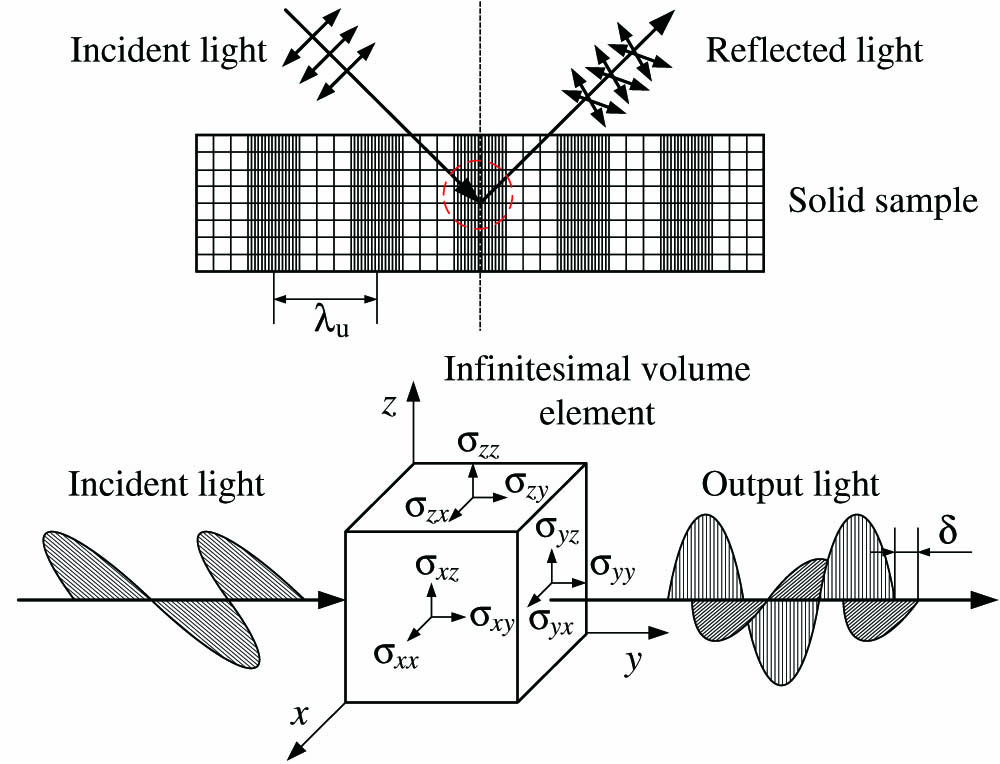
As an ultrasonic wave propagates in a solid, the material particles are compressed and rarified depending on location and time, which results in a nonuniform field of strain in the medium. This strain field will result in an anisotropic distribution of the refractive index through the photoelastic effect, as shown in Fig. 1. When light with a predetermined polarization status passes through the medium, the anisotropic refractive index distribution will lead to variations of the polarization status of the output beam. By detecting the indirect parameters representing the polarization status, information of the strain field caused by the ultrasonic wave can be recovered.

$Schematic diagram of a change in polarization status of light through a solid sample in which an ultrasonic wave propagates. Under the influence of the ultrasonic wave (wavelength λu) propagation, the solid is compressed and rarified depending on location and time, which produces nonuniform stress and strain fields. This leads to an anisotropic distribution of the refractive index and produces a phase difference δ of light through the 3D infinitesimal volume element. The phase difference can be detected by our PIMI system.$

Figure 1.Schematic diagram of a change in polarization status of light through a solid sample in which an ultrasonic wave propagates. Under the influence of the ultrasonic wave (wavelength $λ_{u}$ ) propagation, the solid is compressed and rarified depending on location and time, which produces nonuniform stress and strain fields. This leads to an anisotropic distribution of the refractive index and produces a phase difference $δ$ of light through the 3D infinitesimal volume element. The phase difference can be detected by our PIMI system.

As an ultrasonic wave propagates in a homogeneous, isotropic solid material, the wave equation in displacement can be rewritten as follows^[31,32]: $(λ_{0} + μ_{0}) \nabla (\nabla \cdot u) + μ_{0} \nabla^{2} u = ρ \frac{\partial^{2} u}{\partial t^{2}},$ (1)where $u$ denotes the 3D displacement vector at time $t$ of an arbitrary point in the solid, and $ρ$ is the density of the material. $λ_{0}$ and $μ_{0}$ are the Lame constants, which are related to Young’s modulus $E$ and Poisson’s ratio $ν$ , by $λ_{0} = E ν / [(1 + ν) (1 - 2 ν)]$ and $μ_{0} = E / (2 + 2 ν$ ).

From this 3D displacement vector, one can derive the strain tensor at each point in the solid, $ε_{i j} = \frac{1}{2} (\frac{\partial u_{i}}{\partial x_{j}} + \frac{\partial u_{j}}{\partial x_{i}}) i, j = 1, 2, 3,$ (2)where $ε_{i j}$ is a second-order symmetric tensor and has only six independent constants. The subscript numbers 1, 2, and 3 denote $x$ , $y$ , and $z$ , respectively, namely $x_{1} = x$ , $x_{2} = y$ , and $x_{3} = z$ .

The refractive index at the corresponding point in the medium will be changed by the strain through the photoelastic effect. This is actually the change of size, shape, and orientation of the refractive index ellipsoid if the refractive index of the solid is expressed in terms of the refractive index ellipsoid. Since the strain in the solid is infinitesimally small, the anisotropic photoelastic relation between the strain and the refractive index is usually written as^[33,34] $B_{i j} = P_{i j k l} ε_{k l},$ (3)where $B_{i j}$ is the variation of the inverse dielectric tensor induced by the ultrasonic wave; $P_{i j k l}$ is called the strain-optical or elasto-optic tensor, which is a fourth-order tensor; and $ε_{k l}$ is a second-order symmetric tensor and has only six independent constants. Since $B_{i j}$ and $ε_{k l}$ are symmetric tensors of the second order, the components of $P_{i j k l}$ are not all independent, and the number of independent constants is reduced from 81 to 36, even for the most anisotropic crystal. For an isotropic solid, there are only two independent constants, $P_{11}$ and $P_{12}$ , in the tensor of $P_{i j k l}$ ^[33].

When the light wave propagates through the strain field induced by the ultrasonic wave, it will produce a phase difference $δ$ ^[35], $δ = \frac{2 π}{λ} \int_{0}^{d} Δ n d x_{3},$ (4)where $Δ n$ is the variation of the refractive index, $λ$ is the wavelength of the light wave, and $d$ is the thickness of the solid. Further, let the principal axes of strain (stress) be the axes of the coordinate system, in which the non-diagonal components disappear. If assuming the refractive index change is homogenous along the axes, the relation between the phase difference and strain difference can be expressed as ${\begin{matrix} δ_{11} = \frac{π d_{11} n_{0}^{3}}{λ} (P_{11} - P_{12}) (ε_{22} - ε_{33}) \\ δ_{22} = \frac{π d_{22} n_{0}^{3}}{λ} (P_{11} - P_{12}) (ε_{11} - ε_{33}) \\ δ_{33} = \frac{π d_{33} n_{0}^{3}}{λ} (P_{11} - P_{12}) (ε_{11} - ε_{22}) \end{matrix},$ (5)where $δ_{11}$ , $δ_{22}$ , and $δ_{33}$ are the phase difference in the $x$ , $y$ , and $z$ directions, respectively. $d_{11}$ , $d_{22}$ , and $d_{33}$ are the thickness of the solid in the $x$ , $y$ , and $z$ directions, respectively. $n_{0}$ is the initial refractive index.

When light with a predetermined polarization status, e.g., linear polarization, passes through the medium, the phase difference produced by a certain strain field will lead to the variation of the indirect parameters, which represents the polarization status of the emerging beam. These parameters can be sensed and calculated by the PIMI system, as previously reported by the group^[30,36,37]: ${\begin{cases} S_{0} = I_{dp} (1 + \sin δ) \\ S_{1} = I_{dp} (1 + \sin δ) \cos 2 ϕ \\ S_{2} = \sqrt{2} I_{dp} (1 + \sin δ) \sqrt{\sin 2 ϕ} \cos δ \\ S_{3} = \sqrt{2} I_{dp} (1 + \sin δ) \sqrt{\sin 2 ϕ} \sin δ \end{cases},$ (6)where $I_{dp}$ is the average intensity over all polarization states reflected from each field point. $Φ$ is the polarization angle of the slow axis. The Stokes parameters ( $S_{0}$ , $S_{1}$ , $S_{2}$ , and $S_{3}$ ) are related to the phase difference $δ$ induced by the refractive index change, which was caused by the ultrasonic wave in the medium.

As illustrated in Fig. 2, the experimental setup consists of two parts: an ultrasonic excitation system and a PIMI imaging system, which are used to generate and sense the ultrasonic waves, respectively. The ultrasonic waves were sensed by extracting the variation of optical properties of the sample with and without ultrasonic excitation. In the experiment, we used a quartz glass with the size of $6 mm \times 6 mm \times 20 mm$ as the sample. The piezoelectric ceramic transducer 1 (PZT 1) with resonant frequency of 5 MHz adhered on the end face of the sample was used for generating ultrasonic waves, which were captured by PZT 2 at the opposite end face. The detected ultrasonic signal with PZT 2 was sent to an oscilloscope to monitor the properties of the generated ultrasonic wave in the sample.

Figure 2.Experimental setup of ultrasonic field sensing. It consists of an ultrasonic excitation system and a PIMI system. The excitation system was employed to generate ultrasonic waves in the sample, and the PIMI system was used to image and characterize the ultrasonic field by extracting variations of optical properties of the sample with and without ultrasonic excitation.

A brief description of the PIMI imaging system is included here for the sake of completeness, and more details can be found in Ref. [30]. The system was built by adopting the basic optical microscopic path of an Olympus BX51M microscope and inserting a polarization modulation module with an angle precision of 0.05° in the beam path of illumination light. A Basler (piA2400–17gm) CCD with a pixel resolution of 3.45 μm was used for data acquisition of the optical intensity variation affected by the ultrasonic wave in the sample. The indirect optical images were taken with an illumination wavelength of 532 nm. With regard to the PIMI system, all of the polarization parameters, including the average of polarization intensities $I_{dp}$ , polarization phase difference $\sin δ$ , polarization angle of slow axis $Φ$ , and the Stokes parameters ( $S_{0}$ , $S_{1}$ , $S_{2}$ , and $S_{3}$ ), are related to the phase difference $δ$ induced by the refractive index change, which was caused by the ultrasonic wave in the medium. With these polarization parameters, we can form individual parameter maps or indirect images, as we called them following the pixel coordinates. Consequently, we can study quantitatively the change of the optical properties of solids under the influence of an ultrasonic wave from the indirect images, and the stress and strain fields induced by the ultrasonic field can be recovered accordingly.

As a sinusoidal voltage with amplitude of 20 V and frequency of 5 MHz is applied to PZT 1, an ultrasonic wave with the same frequency was generated in the sample, as indicated by the signal captured by PZT 2. In order to eliminate the effects of surface micro-morphology, defects, and scratches on the ultrasonic field images, the objective of PIMI system was focused on a plane at a depth of about 3 mm beneath the surface of the sample. The PIMI images were taken when the sample was with and without ultrasonic excitation, as shown in Fig. 3.

Figure 3.PIMI images under different ultrasonic conditions (a)–(c) without and (d)–(f) with ultrasonic excitation. (a) and (d) Average of polarization intensities $I_{dp}$ , (b) and (e) polarization phase difference $\sin δ$ , (c) and (f) polarization angle of slow axis $Φ$ .

Figures 3(a)–3(c) show the average of all polarization intensities $I_{dp}$ , polarization phase difference $\sin δ$ , and polarization angle of slow axis $Φ$ without ultrasonic excitation, respectively. In contrast, Figs. 3(d)–3(f) show $I_{dp}$ , $\sin δ$ , and $Φ$ with ultrasonic excitation, respectively. The difference between Figs. 3(a) and 3(d), Figs. 3(b) and 3(e) is trivial while the difference between Figs. 3(c) and 3(f) is obvious. This indicated that the parameter $Φ$ has higher sensitivity to the strain field induced by ultrasonic waves.

The PIMI images of Stokes parameters $S_{0}$ , $S_{1}$ , $S_{2}$ , and $S_{3}$ under different ultrasonic conditions are further shown in Fig. 4. The difference between the images without and with ultrasonic excitation seems to be not distinct, which may imply that these Stokes parameters are not sensitive enough to the ultrasonic field as the parameter $Φ$ .

Figure 4.PIMI images of the Stokes parameters under different ultrasonic conditions (a)–(d) without and (e)–(h) with ultrasonic excitation. (a), (e) $S_{0}$ ; (b), (f) $S_{1}$ ; (c), (g) $S_{2}$ ; (d), (h) $S_{3}$ .

As can be seen from Fig. 4, the size of images varies for Stokes parameters $S_{0}$ , $S_{1}$ , $S_{2}$ , and $S_{3}$ . The reason is that the average light intensity of the whole image was different for different parameters, which leads to a difference of size of the bright area when showing the images with the same color map; even the field of view is the same for all these images.

In order to confirm the sensitivity of the parameter images in Figs. 3 and 4 to the refractive index variation caused by the strain field, the differences between the PIMI images without ultrasonic excitation and those with ultrasonic excitation are obtained by subtracting the images without an ultrasonic wave from those with an ultrasonic wave. The difference images of the parameters $\sin δ$ , $Φ$ , and $S_{1}$ demonstrated sensitivity to the ultrasonic field, as shown in Fig. 5.

Figure 5.Difference between PIMI images without ultrasonic excitation and those with ultrasonic excitation. (a) $\sin δ$ , (b) $Φ$ , and (c) $S_{1}$ .

As described by the theoretical model, the ultrasonic wave induced a variation of strain (stress) fields, leading to the dynamic variation of the refractive index (refractive index ellipsoid) and, therefore, a change of polarization status of the light passing through the medium. The indirect parameter images recorded and calculated by the PIMI system then recover the information of the ultrasonic field, which was imposed on the polarization status of the emerging beam due to the photoelastic effect. The relation between the indirect parameter images and the ultrasonic field is well defined theoretically, which can be used to calculate the ultrasonic field quantitatively in further study. Figure 5 also shows that the parameter $Φ$ is of the highest sensitivity to the ultrasonic field among all the PIMI indirect parameters. Also, due to reflections of light from the upper and lower surfaces and central plane of the sample, the images show a nonuniform distribution of light intensity, which is roughly defined by three circular areas from the center to the edge of the field of view, as shown in Figs. 5(a) and 5(c). These three circular areas with different intensities are due to the different reflectivities and reflection angles from the upper, lower surfaces of the sample and the image plane, which leads to different total light intensities recorded by the CCD at different viewing angles limited by the numerical aperture of the objective. In Fig. 5(b), this effect seems to be eliminated, and only the information from the ultrasonic field was left, which could be an advantage from using the parameter $Φ$ for imaging of ultrasonic fields.

In order to confirm the sensitivity of PIMI images to the ultrasonic field, ultrasonic phases were varied from 0 to $π / 4$ , and the images of $Φ$ were taken, as shown in Fig. 6. The intensity profiles of the PIMI images were varying according to the phase change of the ultrasonic field, as shows in Figs. 6(c) and 6(f). This verified the sensitivity of the PIMI images to the phase of the ultrasonic field.

Figure 6.Image of $Φ$ under different ultrasonic phases. (a) Phase 0, (b) phase $π / 4$ , (c) extracted intensity curves along the line in (a) and (b), (d) difference between (a) and Fig. 3(c), (e) difference between (b) and Fig. 3(c), (f) extracted intensity curves along the line in (d) and (e).

Figure 7 shows the PIMI images of parameters $\sin δ$ , $Φ$ , and $S_{1}$ at different locations in the direction of ultrasonic propagation and their difference images with and without ultrasonic fields. The differences between the PIMI images without ultrasonic excitation and those with ultrasonic excitation can be seen clearly again, especially in the image of $Φ$ . These results are in good agreement with the results in Figs. 3–5. It verifies that the PIMI system can resolve ultrasonic field information, and the parameter image $Φ$ is the most sensitive one.

Figure 7.PIMI images under different ultrasonic conditions (a)–(c) without and (d)–(f) with ultrasonic excitation: (a) and (d) $\sin δ$ , (b) and (e) $Φ$ , (c) and (f) $S_{1}$ . Difference between the PIMI images without ultrasonic excitation and those with ultrasonic excitation: (g) $\sin δ$ , (h) $Φ$ , and (i) $S_{1}$ .

The ultrasonic wavelength in the sample is approximately 1.19 mm if taking the wave velocity of 5950 m/s for compression wave in a quartz glass. Since the field of view ( $2.26 mm \times 1.19 mm$ ) of the system covers only two wavelengths of the ultrasonic wave, there is no obvious wave front of ultrasonic waves in the field of view. But importantly, the variations of optical properties of the sample induced by ultrasonic waves have evidently been observed. In the next work, it is planned to increase the frequency, and thus shorten the ultrasonic wavelength by replacing the piezo transducer with short laser pulses, which can generate high-frequency ultrasonic waves with various shapes according to the optical configuration.

As a proof of concept, the results above demonstrated that the PIMI system can sense the ultrasonic field by taking images of the indirect parameters, which represent the polarization status of the light affected by the refractive index variations in the sample. The relation between these parameters is well defined in theory, and the ultrasonic field can be further studied quantitatively with the proposed theoretical model. As shown in the experimental results, the image of parameter $Φ$ shows the highest sensitivity to the ultrasonic field. As with all optical ultrasonic detection methods mentioned above, the PIMI method has limitations in reconstruction of 3D ultrasonic fields caused by light deflection and cannot replace conventional hydrophone measurements^[25]. However, this method, which has potential for non-contact and rapid imaging of ultrasonic fields with high spatial resolution, is still attractive.

In summary, by using the PIMI method, signals of ultrasonic waves transmitted in a sample have been clearly picked up in a non-contact way. The structural anisotropy associated with the stress and strain generated by the ultrasonic wave propagation can cause variation of the refractive index, which leads to the variations of the polarization status of the light passing through the medium. The PIMI method measures the indirect parameters, such as $\sin δ$ , $Φ$ , and the Stokes parameters, which are directly representing the polarization status of light. The experimental result proved that the indirect parameter image of $Φ$ is highly sensitive to the ultrasonic field. Also, as the relation between the indirect parameter images and the ultrasonic field is well defined in the theoretical model, the ultrasonic field can be further investigated quantitatively. This study provided a theoretical foundation and experimental proof of concept to image an ultrasonic field with the PIMI method. It is of potential for non-contact and rapid imaging of ultrasonic fields with high spatial resolution, which is useful in applications such as photoacoustic imaging.

References

[1] T. Kundu. Ultrasonic Nondestructive Evaluation: Engineering and Biological Material Characterization(2003).

[2] K. Sun, L. Yuan, Z. Shen, Z. Xu, Q. Zhu, X. Ni, J. Lu. Appl. Opt., 53, 2366(2014).

[3] K. Xia, X. Zhai, Z. Xie, K. Zhou, Y. Feng, G. Zhang, C. Li. Chin. Opt. Lett., 16, 121701(2018).

[4] S. E. Park, T. R. Shrout. IEEE Trans. Ultrason. Ferroelectr. Freq. Control, 44, 1140(1997).

[5] N. Ichinose, N. Miyamoto, S. Takahashi. J. Eur. Ceram. Soc., 24, 1681(2004).

[6] S. K. Tiwari, B. S. Satyanarayana, A. G. Pai, S. K. Tiwari. Defence Sci. J., 59, 627(2009).

[7] A. Novell, M. Legros, J. M. Grégoire, P. A. Dayton, A. Bouakaz. Phys. Med. Biol., 59, 4879(2014).

[8] Y. Zhao, L. Cui, J. Sun, J. Ma, Z. Jia. Chin. Opt. Lett., 12, S11102(2014).

[9] M. C. Bhardwaj. 16th World Conference on Nondestructive(2004).

[10] G. Paltauf, R. Nuster, M. Haltmeier, P. Burgholzer. Appl. Opt., 46, 3352(2007).

[11] S. A. Guerra, A. Guerra, Q. Duque, V. Vengupalan. Appl. Phys. Lett., 85, 5772(2004).