
Yong Chen, Hongguang Guo, Yapeng Ai. Single Image Dehazing of Multiscale Deep-Learning Based on Dual-Domain Decomposition[J]. Acta Optica Sinica, 2020, 40(2): 0210003
- Acta Optica Sinica
- Vol. 40, Issue 2, 0210003 (2020)
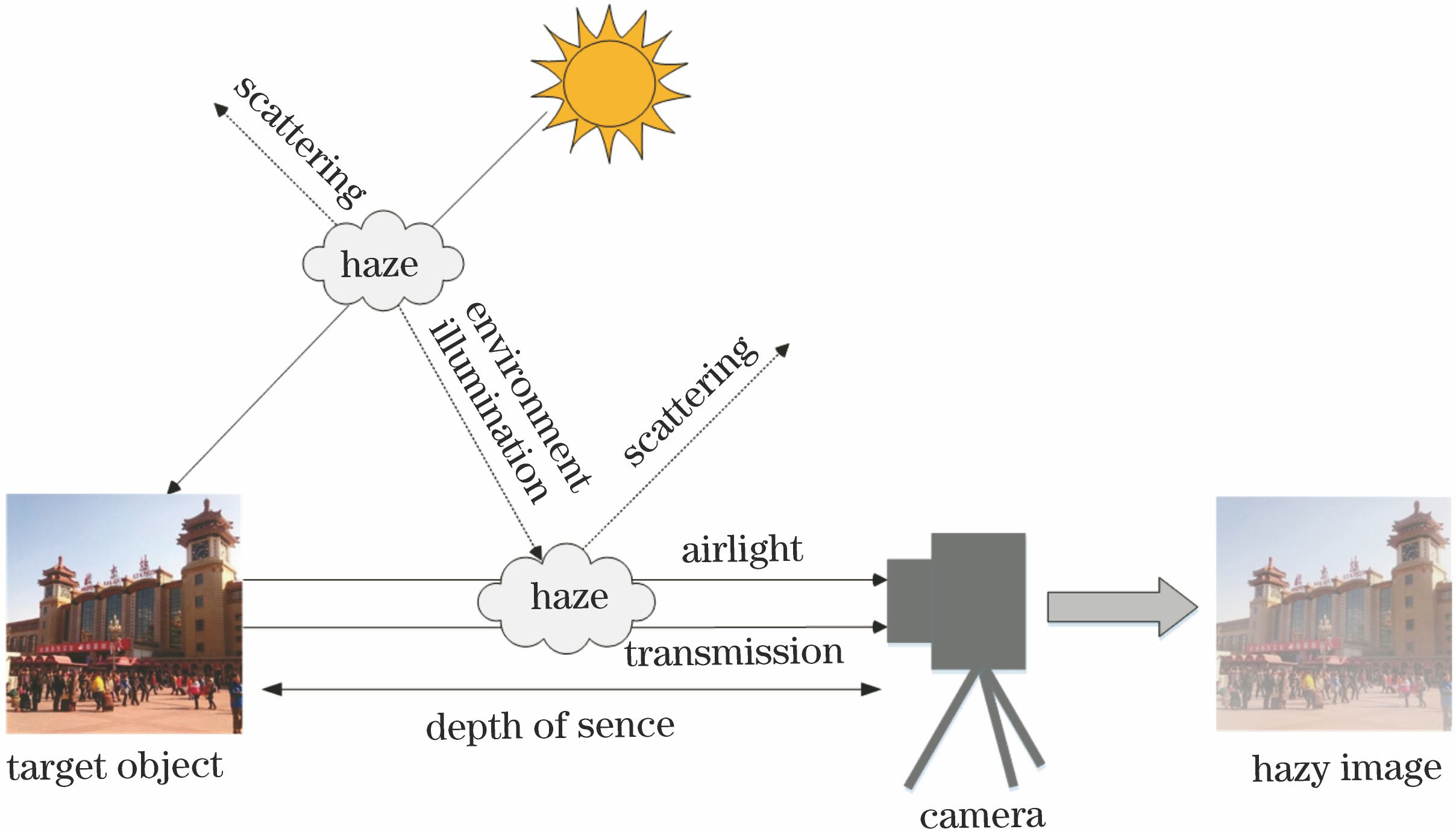
Fig. 1. Physical model of atmospheric scattering
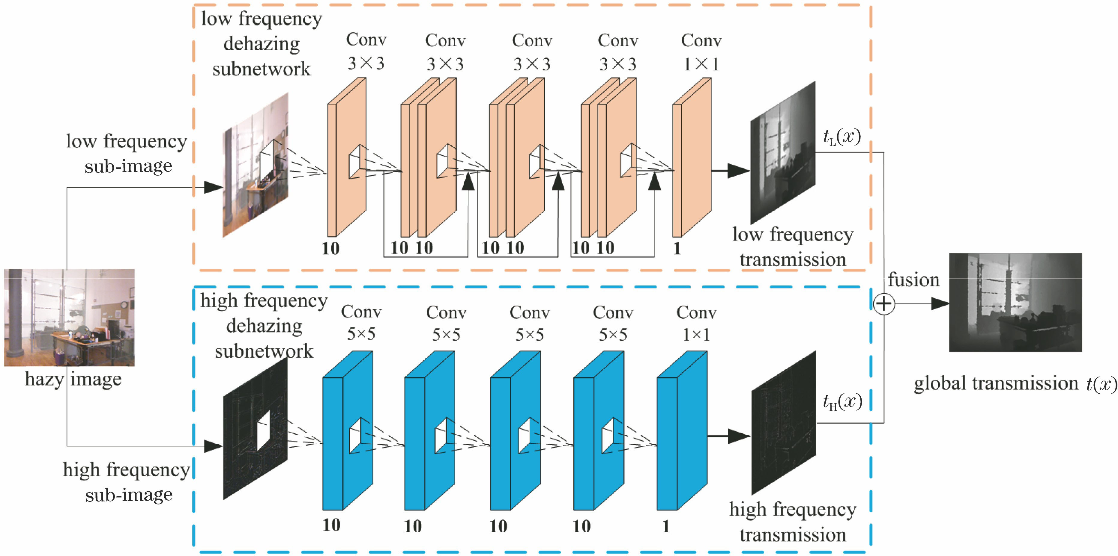
Fig. 2. Schematic of single image dehazing model of multiscale deep-learning based on dual-domain decomposition
Fig. 3. Original image and its high- and low-frequency sub-images. (a) Original image; (b) high-frequency sub-image; (c) low-frequency sub-image
Fig. 4. Comparison of activation functions. (a) ReLU function; (b) PReLU function
Fig. 5. Schematic of single image dehazing algorithm of multiscale deep-learning based on dual-domain decomposition
Fig. 6. Outdoor hazy images and corresponding scene transmission labels after depth map preprocessing
Fig. 7. Experimental results of synthetic hazy images processed by different methods. (a) Synthetic hazy images; (b) stardard dehazed images; (c) method in Ref. [6]; (d) method in Ref. [9]; (e) method in Ref. [11]; (f) method in Ref. [12]; (g) method in Ref. [13]; (h) proposed method
Fig. 8. Experimental results of real natural hazy images processed by different methods. (a) Hazy images; (b) method in Ref. [6]; (c) method in Ref. [9]; (d) method in Ref. [11]; (e) method in Ref. [12]; (f) method in Ref. [13]; (g) proposed method
| |||||||||||||||||||||||||||||||||||||||||||||||||||||||||||||||||||||||||||||||||||||||||||||||||||||||||||||||||||||||||||||
Table 1. Analysis of experimental results of synthetic hazy images processed by different methods
| |||||||||||||||||||||||||||||||||||||||||||||||||||||||||||||||||||||||||||||||||||||||||||||||||||||||||||||||||||||||||||||||||||||||||||||||||||||||||||||||||||||||||||||||||||
Table 2. Analysis of experimental results of real hazy images processed by different methods

Set citation alerts for the article
Please enter your email address
© Copyright 2018-2021 | Chinese Laser Press. All Rights Reserved 沪ICP备15018463号-20