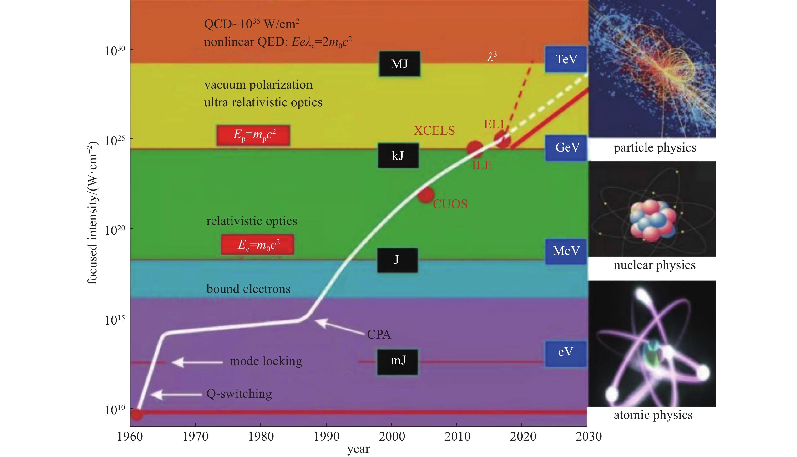
Fig. 1. The development of laser intensity and the corresponding physical research

Fig. 2. Quantum and intensity parameters of LUXE compared to Astra-Gemini and Eli-NP^[24]

Fig. 3. Schwinger tunneling^[31]

Fig. 4. Diagram of multiphoton absorption^[34]

Fig. 5. General form of an oscillating electric field with double-pulse structure. The pulses are characterized by their frequency ω_j , intensity parameter ξ_j and number of plateau cycles N_j( j ∈{1, 2}) and have variable time delay δ^[49]

Fig. 6. Transversal momentum distributions of particles created in an electric double pulse with ξ₁=ξ₂=1, ω=0.49072m, N₁=N₂=6, and time delay δ=0 (blue solid curve) or δ=π/2m (gray dashed curve). The longitudinal momentum component along the field direction vanishes, p_y=0^[49]

Fig. 7. Longitudinal momentum distribution of electrons created in a bifrequent electric field with ξ₁=1, ξ₂=0.1, N=7, and ω=0.49072m [see Eq. (19)]. The black solid (red dashed) curve refersto a relative phase of φ=0 (φ=π/2). The transverse momentumvanishes, p_x=0^[49]

Fig. 8. Phase-of-the-phase spectra for the electron created in a bifrequent electric field with ξ₁=1, ξ₂=0.1, N=7, and ω=0.49072m. Left panel: Φ₁; right panel: Φ₂ (each measured in rad with −π≤Φ_ℓ≤π, as indicated by the color coding)^[54]

Fig. 9. The Fourier transform of the frequency modulated electric field, where the values of modulation parameter (ω_m, b) are (0.01, 1.52) for the upper panel and (0.009, 9.52) for the lower panel. And the values of dominant frequency peaks are shown. Other field parameters are E₀=0.1E_cr, τ =100/m, ω=0.5m^[60]

Fig. 10. The number of the created e⁻e⁺ pairs under the modulated electric field. The electric field strength E₀=0.1E_cr, and the laser frequency ω=0.5m. The other parameters τ=100/m, b and ω_m are variables^[60]

Fig. 11. The number density of created electron-positron pairs as a function of field frequency ω. The oscillating structures are related to the n-photon thresholds. The upper line corresponds to E₀=0.1E_cr and the lower line corresponds to E₀=0.01E_cr. Other field parameters are τ =100/m. Note that there is no frequency modulation, i.e., b=0^[60]

Fig. 12. (a) Sketch of the temporal behavior of the chirped electric field pulse E(t) used in this work. (b) The Page-Lampard S_PL(ω,t) spectrum taken at different time for E(t) with ω₀=2c² andb=c². The bottom graph is the traditional spectrum S_T(ω) of E(t)^[62]

Fig. 13. (a) Contour plot of the temporal derivative of the energy spectrum of the created number of positron |C_p;u(t)|² as a function of the positron energy e_p. (b) The Page-Lampard spectrum S_PL(ω,t) of the external electric force field E(t). Other parameters are T_on=0.01 a.u., T_off=0.01 a.u., T=0.025 a.u., ω₀=2c² and b=c², E₀=0.005c^3[62]

Fig. 14. The steady-state pair-creation rate Γ as a function of the effective width σ of four electric field configurations with a singly peaked spatial envelope^[69]

Fig. 15. Contour profile plot of the space-time structure of the potential with M=8. Other parameters are D=20/c, d=1/c, W=0.5/c, V₀=1.3c², and ω=1.2c². The spatial size of the simulation is L=1.2^[71]

Fig. 16. The number of created particles for different values of M. The other parameters of the potential are given as D=20/c, d=1/c, W=0.5/c, V₀=1.3c², ω=1.2c², N_x=4096, and L=4.8^[71]

Fig. 17. Contour profile plot of the spacetime structure of the potential well. Panel (a) is for φ=0, panel (b) is for φ=π/2, panel (c) is for φ=π, and panel (d) is for φ=3π/2. The simulation time is set to t=50π/c². Other parameters are D₀=10λ_c, V₀=2.53c², and ω₀=0.04c², the spatial size is L=2.5^[72]

Fig. 18. Number of created electrons as a function of phase φ over a period of 2π. The simulation time is set to t = 50π/c². Other parameters are the same as in Fig. 17 ^[72]

Fig. 19. Instantaneous eigenvalues of the potential well over time. Other parameters are the same as those in Fig.18^[72]

Fig. 20. Sketch of the electric field configuration based solely on a supercritical field at x= 0 (top panel). In the bottom panel, a second (control) field at x=−d is added^[81]

Fig. 21. Quantitative representation of Fig. 20, where V_s=2.5mc², V_c=0.25mc², w=0.075ħ/αmc, d=0.2ħ/αmc, the interaction time was t=0.045ħ/α²mc² and α is the fine structure constant^[81]

Fig. 22. Sketch of the setup for a vacuum mode as a carrier of information. The left inset show the time dependence of an electric pulse that is spatially localized at a distant L from the receiver^[84]

Fig. 23. The open circles show the growth of the number density of created positrons N(E, t). For comparison, the solid line is the prediction according to Eq. (32). The displayed pulse durations of the sender’s field are in 10⁻³ atomic units^[84]

Fig. 24. The growth of the energy of the created electrons during the interaction with a chirped external electric field. L=2.4 a.u. and the other parameters are b=300c², ω=2.8c², τ=5.325×10^–4 a.u., t₁=0.004 a.u. and F₀=5c^3[87]

Fig. 25. The growth of the total energy of the created electrons during the interaction with a chirped external field. L=2.4 and the other parameters are V₀=5c², W=0.5/c, D=0.6 a.u.andb=300c², ω=2.8c², τ=5.325×10^–4 a.u. and t₁=0.004 a.u.^[87]

Table 1. Operational parameters of the three HPLS beam lines at ELI-NP ^[19]

Table 2. The number density for different selected sets of modulation constants (ω_m, b)，see the points marked in Fig. 10 ^[60]

Table 3. The mean pair creation rate Γ_M for different values of M^[71]