• Chinese Optics Letters
  • Vol. 19, Issue 7, 073201 (2021)
Jiu Tang, Guizhong Zhang*, Yufei He, Xin Ding, and Jianquan Yao
Author Affiliations
  • College of Precision Instrument and Optoelectronics Engineering, Tianjin University; Key Laboratory of Optoelectronic Information Technology, Ministry of Education, Tianjin 300072, China
  • show less
    DOI: 10.3788/COL202119.073201 Cite this Article Set citation alerts
    Jiu Tang, Guizhong Zhang, Yufei He, Xin Ding, Jianquan Yao. Scattering-amplitude phase in spiderlike photoelectron momentum distributions[J]. Chinese Optics Letters, 2021, 19(7): 073201 Copy Citation Text show less
    Photoelectron momentum distributions of hydrogen atoms simulated by (a)–(c) the semiclassical rescattering model (SRM, α is set to zero; red dots on the interference minima are just for guiding the eyes) and (d)–(f) TDSE. Because there are not many optical cycles in the pulse, the TDSE results are asymmetric with respect to the px = 0 axis. The top two panels correspond to wavelengths of (a), (d) λ=1900 nm, (b), (e) λ=2000 nm, and (c), (f) λ=2100 nm, respectively. (g) Typical trajectories that form the spiderlike structure in the SRM: the parent ion is at the origin of the axis. The pink curve is the reference trajectory, and the red curve is the signal trajectory. A scattering angle of 5° is assumed for the signal trajectory. (h) Cut-plot curves taken at px = 0.4 a.u. for the SRM (blue) and TDSE (red), and the cut positions are marked by the colored vertical lines in (b) and (e). Intensity of the laser pulse is I = 4×10¹³ W/cm2, and the pulse duration is two optical cycles.
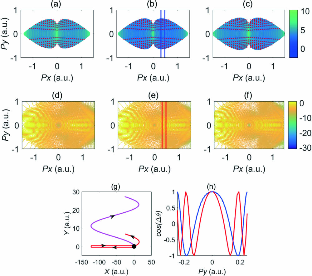
    Fig. 1. Photoelectron momentum distributions of hydrogen atoms simulated by (a)–(c) the semiclassical rescattering model (SRM, α is set to zero; red dots on the interference minima are just for guiding the eyes) and (d)–(f) TDSE. Because there are not many optical cycles in the pulse, the TDSE results are asymmetric with respect to the px = 0 axis. The top two panels correspond to wavelengths of (a), (d) λ=1900nm, (b), (e) λ=2000nm, and (c), (f) λ=2100nm, respectively. (g) Typical trajectories that form the spiderlike structure in the SRM: the parent ion is at the origin of the axis. The pink curve is the reference trajectory, and the red curve is the signal trajectory. A scattering angle of 5° is assumed for the signal trajectory. (h) Cut-plot curves taken at px = 0.4 a.u. for the SRM (blue) and TDSE (red), and the cut positions are marked by the colored vertical lines in (b) and (e). Intensity of the laser pulse is I = 4×10¹³W/cm2, and the pulse duration is two optical cycles.
    Spiderlike structures numerically obtained by the SRM. The patterns correspond to phase values of (a) α=0, (b) π/20, (c) π/10, (d) 3π/20, (e) π/5, (f) π/4, and (g) 3π/10, respectively. (h) Cut-plot curves are taken at px = 0.4 a.u. from the spiderlike patterns in (a) (blue solid curve), (b) (red solid curve), (c) (green solid curve), (d) (black solid curve), (e) (blue dotted curve), (f) (red dotted curve), and (g) (green dotted curve), respectively. The cut positions are marked by the colored vertical lines in (a)–(g). The laser parameters are the same as in Fig. 1.
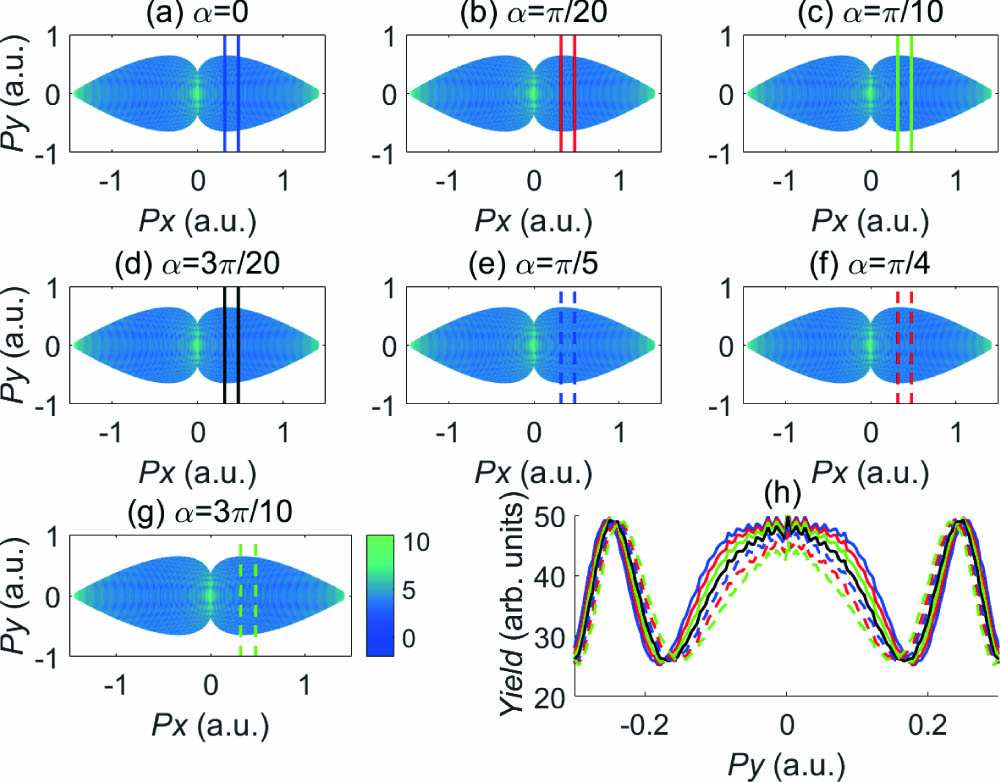
    Fig. 2. Spiderlike structures numerically obtained by the SRM. The patterns correspond to phase values of (a) α=0, (b) π/20, (c) π/10, (d) 3π/20, (e) π/5, (f) π/4, and (g) 3π/10, respectively. (h) Cut-plot curves are taken at px = 0.4 a.u. from the spiderlike patterns in (a) (blue solid curve), (b) (red solid curve), (c) (green solid curve), (d) (black solid curve), (e) (blue dotted curve), (f) (red dotted curve), and (g) (green dotted curve), respectively. The cut positions are marked by the colored vertical lines in (a)–(g). The laser parameters are the same as in Fig. 1.
    (a) Blue area presents the tunneling time range of signal electron wavepackets and reference electron wavepackets involved in the spiderlike structures. The red curve presents the rescattering time range of signal electron wavepackets. (b) Variations of the time difference between rescattering of the signal electron and ionization of the reference electron with px. The red circles, blue circles, and black pluses represent the time difference extracted by fitting the cut-plot curves of the spiderlike structure using Eq. (9), the time differences obtained by the SRM, and the time differences calculated by the saddle-point equations, respectively.
    Fig. 3. (a) Blue area presents the tunneling time range of signal electron wavepackets and reference electron wavepackets involved in the spiderlike structures. The red curve presents the rescattering time range of signal electron wavepackets. (b) Variations of the time difference between rescattering of the signal electron and ionization of the reference electron with px. The red circles, blue circles, and black pluses represent the time difference extracted by fitting the cut-plot curves of the spiderlike structure using Eq. (9), the time differences obtained by the SRM, and the time differences calculated by the saddle-point equations, respectively.
    (a) Cut-plot curves are taken at px = 0.4 a.u. from the spiderlike patterns corresponding to α=0 (blue curve), π/10 (red curve), π/5 (green curve), and 3π/10 (black curve), respectively. The first, second, and third interference minimum positions are marked by black dotted circles. (b) Variations of the interference minimum positions (values of transverse momenta or py) of the cut-plot curves taken at px = 0.4 a.u. with α. The first, second, and third interference minimum positions calculated using Eq. (9) are marked by blue circles. For comparison, the corresponding positions calculated by the SRM are shown by red pluses, red crosses, and red star symbols.
    Fig. 4. (a) Cut-plot curves are taken at px = 0.4 a.u. from the spiderlike patterns corresponding to α=0 (blue curve), π/10 (red curve), π/5 (green curve), and 3π/10 (black curve), respectively. The first, second, and third interference minimum positions are marked by black dotted circles. (b) Variations of the interference minimum positions (values of transverse momenta or py) of the cut-plot curves taken at px = 0.4 a.u. with α. The first, second, and third interference minimum positions calculated using Eq. (9) are marked by blue circles. For comparison, the corresponding positions calculated by the SRM are shown by red pluses, red crosses, and red star symbols.
    (a) Values of phase α extracted from the cut-plot curves simulated by TDSE, plotted as a function of py. (b) Cut-plot curves taken at px = 0.4 a.u. The red dashed curve represents the curve obtained from TDSE. The blue solid curve represents the modified results of Fig. 1(a) after considering a phase value given in Fig. 5(a) in SRM.
    Fig. 5. (a) Values of phase α extracted from the cut-plot curves simulated by TDSE, plotted as a function of py. (b) Cut-plot curves taken at px = 0.4 a.u. The red dashed curve represents the curve obtained from TDSE. The blue solid curve represents the modified results of Fig. 1(a) after considering a phase value given in Fig. 5(a) in SRM.
    Jiu Tang, Guizhong Zhang, Yufei He, Xin Ding, Jianquan Yao. Scattering-amplitude phase in spiderlike photoelectron momentum distributions[J]. Chinese Optics Letters, 2021, 19(7): 073201
    Download Citation