Detection of Anthracnose in Camellia Oleifera Based on Laser-Induced Breakdown Spectroscopy

Yande Liu; Xue Gao; Mengjie Cheng; Zhaoguo Hou; Xiaodong Lin; Jia Xu

doi:10.3788/LOP57.093006

Journals >Laser & Optoelectronics Progress >Volume 57 >Issue 9 >Page 093006 > Article

Laser & Optoelectronics Progress
Vol. 57, Issue 9, 093006 (2020)

Detection of Anthracnose in Camellia Oleifera Based on Laser-Induced Breakdown Spectroscopy

Yande Liu^*, Xue Gao, Mengjie Cheng, Zhaoguo Hou, Xiaodong Lin, and Jia Xu

Author Affiliations

Institute of Optics Mechanics Electronics Technology and Application, East China Jiaotong University, Nanchang, Jiangxi 330013, China

show less

DOI: 10.3788/LOP57.093006 Cite this Article Set citation alerts

Yande Liu, Xue Gao, Mengjie Cheng, Zhaoguo Hou, Xiaodong Lin, Jia Xu. Detection of Anthracnose in Camellia Oleifera Based on Laser-Induced Breakdown Spectroscopy[J]. Laser & Optoelectronics Progress, 2020, 57(9): 093006 Copy Citation Text

show less

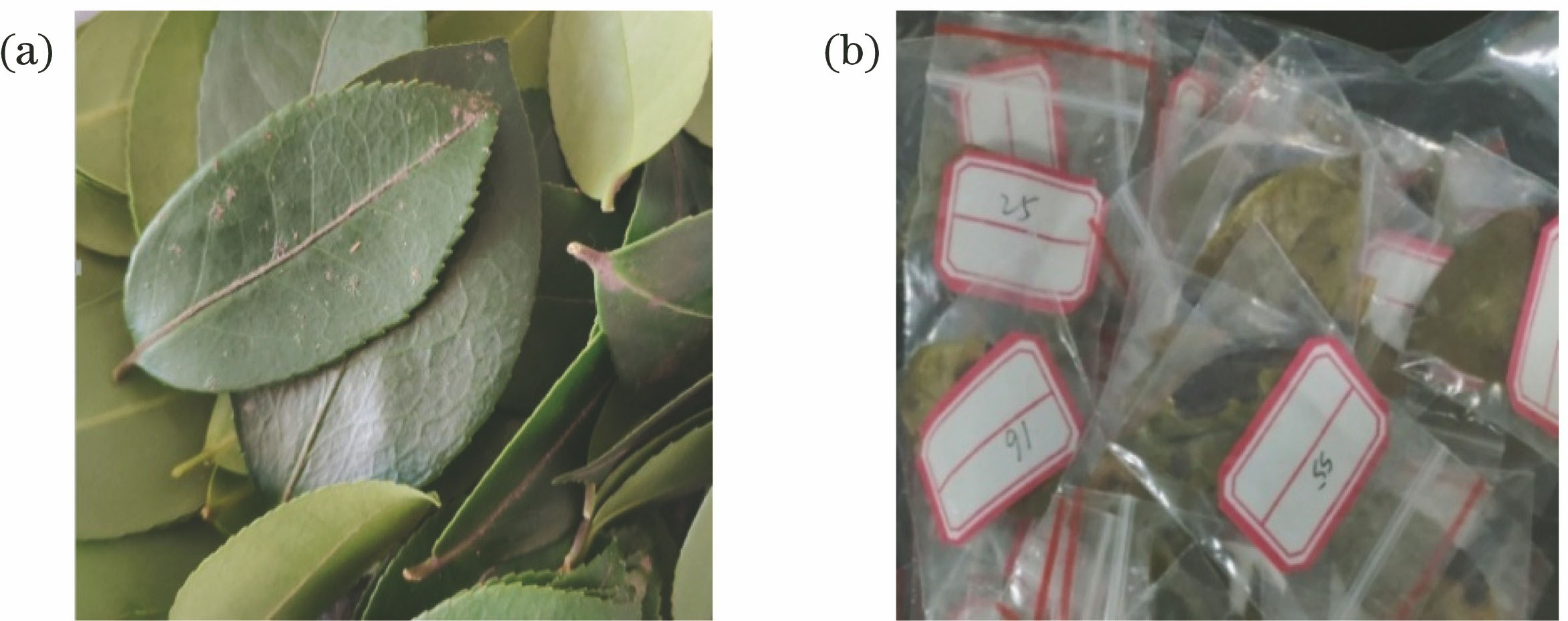
Fig. 1. Sample of camellia oleifera leaves. (a) Healthy camellia oleifera leaves; (b) infected anthracnose camellia oleifera leaves

Download full size

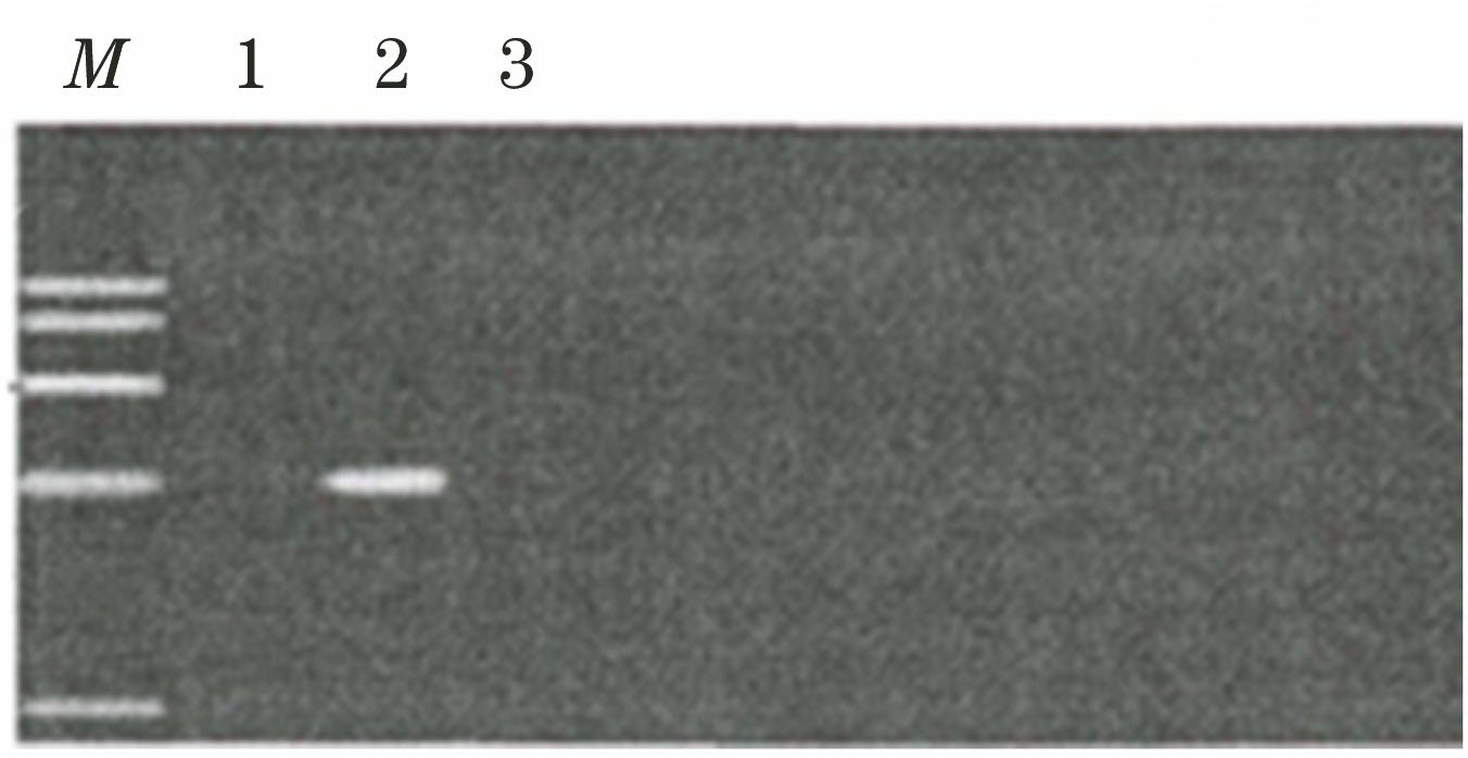
Fig. 2. PCR test results of camellia oleifera leaves

Download full size

Fig. 3. Original spectrum of camellia oleifera leaves after interception

Download full size

Fig. 4. Working curve of standard solution. (a) Healthy camellia oleifera leaves; (b) infected anthracnose camellia oleifera leaves

Download full size

Fig. 5. Location of characteristic line of Mn element

Download full size

Fig. 6. Comparison before and after data smoothing

Download full size

Fig. 7. PLS model and prediction model of Mn element after 7-point data smoothing and first derivative de-noising. (a) PLS model; (b)prediction model

Download full size

Fig. 8. Best sub-interval selected by the iPLS model. (a) Spectral graph of the 24th interval with RMSECV; (b) spectral graph corresponding to the 6th sub-interval

Download full size

Fig. 9. iPLS modeling set scatter diagram

Download full size

Fig. 10. iPLS prediction set scatter diagram

Download full size

Testcondition	Wavelength /nm	Lampcurrent /mA	Acetylene flowrate /(L·min^-1)	Airflowrate /(L·min^-1)	Slitwidth /nm
Parameter	279.5	3	1.3	7.5	0.2

Table 1. Determination conditions of Mn element

Sample	Category	Numberof samples	Rangevalue /(mg·mg^-1)	Averagevalue /(mg·mg^-1)
Healthy camelliaoleifera leaves	calibration set	181	1.0600-4.2570	2.2919
Healthy camelliaoleifera leaves	prediction set	59	1.4610-3.7240	2.2767
Camellia oleifera leaves with anthracnose	calibration set	157	0.7990-3.3290	1.4476
Camellia oleifera leaves with anthracnose	prediction set	51	1.0680-2.7880	1.3581

Table 2. Division of samples

Spectral pretreatmentmethod	Evaluationindex	Beforesmoothing	5 pointssmoothing	7 pointssmoothing	9 pointssmoothing
	R_C	0.8461	0.8621	0.8956	0.8760
Original	RMSECV /(μg·mg^-1)	0.2575	0.2499	0.2204	0.2433
	R_P	0.8195	0.8212	0.8540	0.8315
	RMSEP /(μg·mg^-1)	0.2769	0.2658	0.2548	0.2591
	R_C	0.8534	0.8562	0.8648	0.8605
Denoising	RMSECV /(μg·mg^-1)	0.2434	0.2375	0.2403	0.2482
	R_P	0.8162	0.8196	0.8329	0.8142
	RMSEP /(μg·mg^-1)	0.2553	0.2469	0.2373	0.2499
	R_C	0.8345	0.8440	0.8840	0.8396
Baseline correction	RMSECV /(μg·mg^-1)	0.2875	0.2570	0.1770	0.2764
	R_P /(μg·mg^-1)	0.8010	0.8219	0.8333	0.8019
	RMSEP /(μg·mg^-1)	0.3169	0.2722	0.2524	0.2911
	R_C	0.8584	0.8947	0.9025	0.8892
First derivativede-noising	RMSECV /(μg·mg^-1)	0.2414	0.2206	0.2192	0.2227
	R_P	0.8215	0.8519	0.8882	0.8352
	RMSEP /(μg·mg^-1)	0.2692	0.2474	0.2356	0.2339
	R_C	0.8523	0.8521	0.8507	0.8619
Second derivativede-noising	RMSECV /(μg·mg^-1)	0.2528	0.2532	0.2569	0.2354
	R_P	0.8190	0.8150	0.8377	0.8323
	RMSEP /(μg·mg^-1)	0.2784	0.2791	0.2774	0.2802
	R_C	0.8323	0.8389	0.8429	0.8413
Normalization	RMSECV /(μg·mg^-1)	0.2829	0.2705	0.2711	0.2514
	R_P	0.8189	0.8106	0.8254	0.8177
	RMSEP /(μg·mg^-1)	0.3062	0.3098	0.2955	0.3016

Table 3. PLS model results of smoothed data processed by different preprocessing methods

Interval number	Optimum principal component	RMSECV /(μg·mg^-1)	R	Optimum interval
1	7	0.2770	0.8304	1
2	9	0.2580	0.8548	1
3	10	0.2360	0.8807	1
4	12	0.2200	0.8966	1
5	6	0.2510	0.8632	2
6	6	0.2490	0.8660	2
7	6	0.2560	0.8577	2
8	6	0.2550	0.8589	2
9	7	0.2330	0.8843	3
10	8	0.2350	0.8832	3
11	7	0.2380	0.8797	3
12	7	0.2400	0.8769	3
13	7	0.2200	0.8966	4
14	6	0.2260	0.8918	4
15	7	0.2240	0.8931	4
16	7	0.2270	0.8899	4
17	6	0.2220	0.8945	5
18	6	0.2210	0.8961	5
19	7	0.2170	0.8999	5
20	8	0.2200	0.8979	5
21	6	0.2350	0.8816	6
22	8	0.2160	0.9016	6
23	8	0.2160	0.9013	6
24	8	0.2090	0.9076	6
25	6	0.2280	0.8889	7
26	7	0.2100	0.9068	7
27	6	0.2140	0.9027	7
28	6	0.2090	0.9067	7
29	8	0.2700	0.8414	7
30	8	0.2190	0.8996	8

Table 4. iPLS modeling analysis results

Download Citation

Set citation alerts for the article

Tools

Set citation alerts for the article

Save the article for my favorites

Paper Information