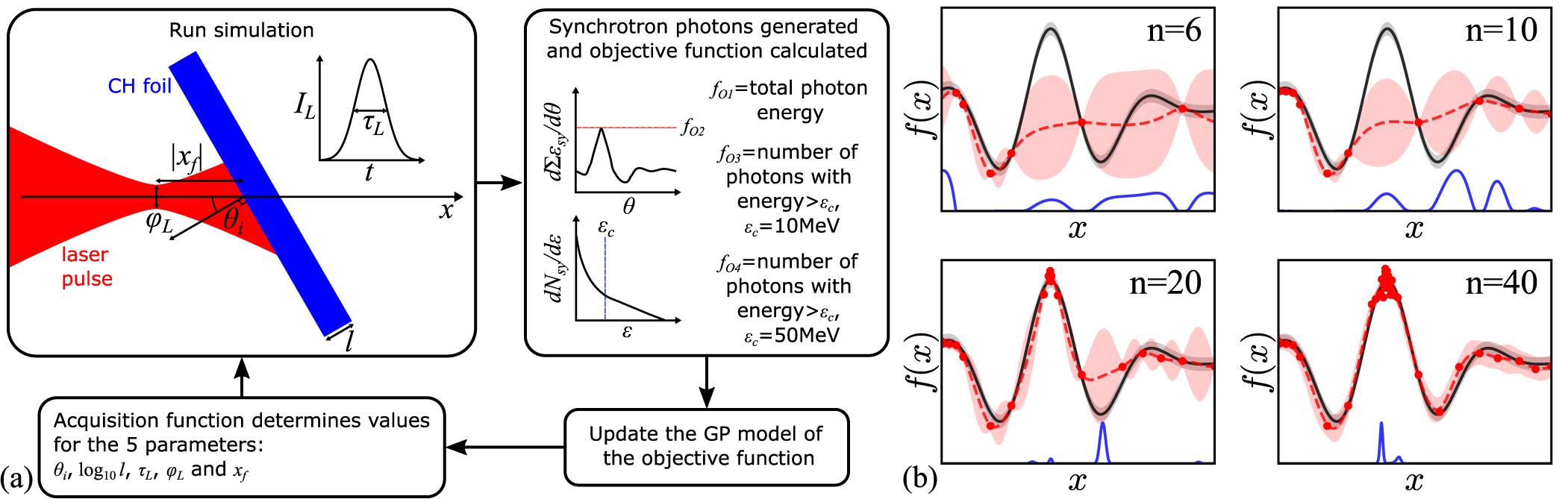
Fig. 1. (a) The Bayesian optimization loop and schematic of the simulation setup. The synchrotron photon energy spectrum () and angle-resolved yield () generated in each simulation are depicted to illustrate several of the objective functions. (b) An example of Bayesian optimization of a noisy 1D function showing the true function (black), the model (red) and the acquisition function (blue) for different numbers of iterations (n).

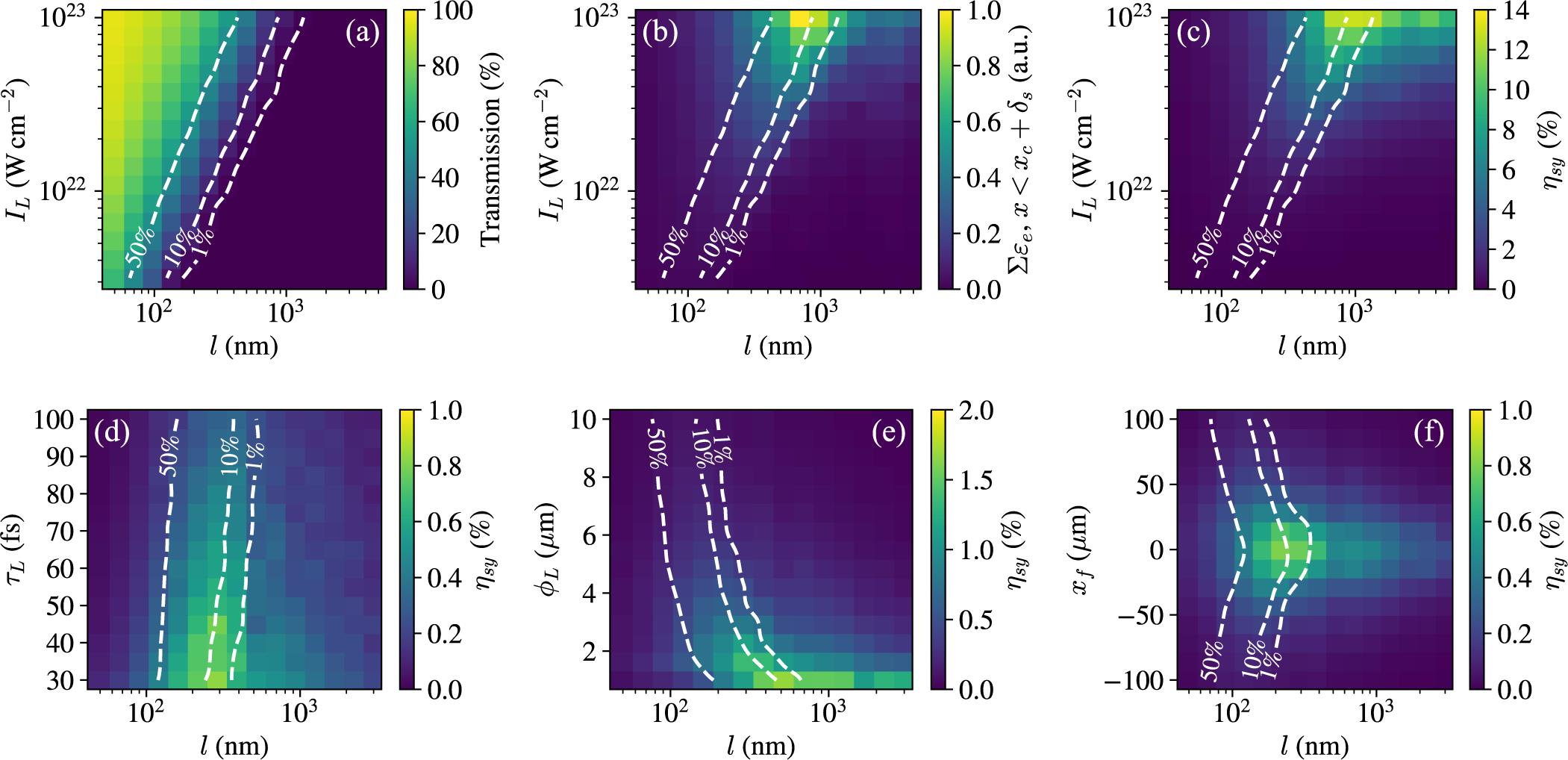
Fig. 2. (a) Percentage transmission of the laser pulse, (b) total electron energy in front of the plasma critical surface and in the laser skin depth averaged over the period of synchrotron emission and (c) laser-to-synchrotron photon energy conversion efficiency, all for varying target thickness and laser intensity. (d)–(f) Laser-to-synchrotron photon energy conversion efficiency for varying pulse duration, focal spot size and defocus, respectively, with target thickness.

Fig. 3. Scaling of the laser-to-synchrotron energy conversion efficiency with (a) peak laser intensity, (b) pulse duration and (c) focal spot FWHM, for varying target thickness. Power law fits are shown for the optimum target thicknesses (black) and for the thickest targets used (red; for (a) and for (b) and (c)).

Fig. 4. (a) Laser-to-synchrotron photon energy conversion efficiency for varying angle-of-incidence and target thickness. (b) Electron spectra, sampled over the whole simulation space, averaged over the period of synchrotron emission for a 200 nm foil at normal and 45° incidence, and (c) the corresponding time-averaged spectra.

Fig. 5. (a) Laser-to-bremsstrahlung radiation energy conversion efficiency for varying laser intensity and target thickness. (b) Energy spectra for bremsstrahlung photons (solid) and synchrotron photons (dotted) for different target thicknesses. (c) The rate of energy conversion to bremsstrahlung radiation.

Fig. 6. Synchrotron and bremsstrahlung radiation for the objective function optima in Table 1, for which fsmW cm⁻². (a) Synchrotron photon energy spectra, (b) bremsstrahlung photon energy spectra and (c) angular profiles of total emitted synchrotron photon energy.

Fig. 7. Synchrotron and bremsstrahlung radiation for the objective function optima in Table 2, for which fsmW cm⁻². (a) Synchrotron photon energy spectra, (b) bremsstrahlung photon energy spectra and (c) angular profiles of total emitted synchrotron photon energy.

Fig. 8. (a) Maximum value of as a function of the angle-of-incidence for synchrotron photons emitted in angular ranges (black) and (blue), where m, W cm⁻², m, fs and . The optima in Figure 6 are also shown (diamonds). (b) Total energy in electrons more than 10 MeV in a local intensity more than 10²¹ W cm⁻² propagating with angle in the ranges (dashed) and (solid) averaged over the period of synchrotron emission. (c) Energy-weighted mean angle between the electron trajectory and the propagation direction of the local electromagnetic field (left-hand axis) and mean electron quantum parameter (right-hand axis) for each group of electrons in (b). (d)–(f) The electron density for , 22.5° and 60°, respectively, where the total momentum of fast electrons (arrows) and the W cm⁻² contour (red) are also shown.

Fig. 9. 3D simulation results for synchrotron photon emission for different laser light polarization states. Peak angle-resolved synchrotron energy emitted in each direction for (a) p-polarization, (b) s-polarization and (c) left-hand and right-hand circular polarization. (d)–(f) Conversion efficiency to synchrotron radiation for p-, s- and both left-hand and right-hand circular polarization, respectively.

Fig. 10. Angular profiles of the total energy of synchrotron emission in the forward direction () in 3D simulations for different laser light polarization states and angles-of-incidence.

Table 1. The objective functions maximized with Bayesian optimization and the parameters of the found optimum for each.

Table 2. The objective functions used for optimization with laser intensity of fsmW cm⁻², and the parameters of the found optima.