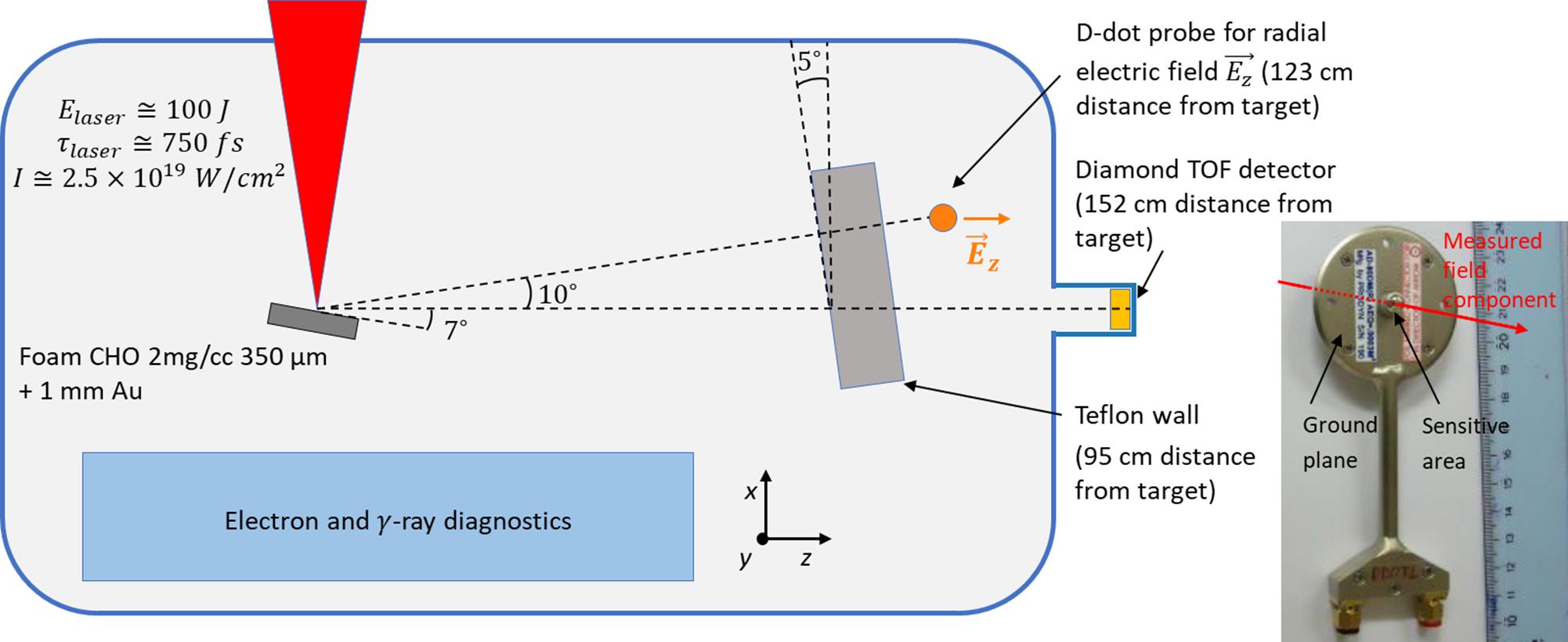
Fig. 1. Experimental setup during the campaign. The focused laser pulse irradiated the solid target, tilted by with respect to the laser axis. Electron and -ray diagnostics were placed in the laser forward direction, whereas the EMP field probe was placed at about from the laser axis at a distance of 123 cm from the interaction point. The ions accelerated by the interaction were detected by means of a diamond TOF diagnostic that was elevated above the Teflon ( from the laser axis, 152 cm away from the target). The photograph shows the D-dot probe used in the experiment.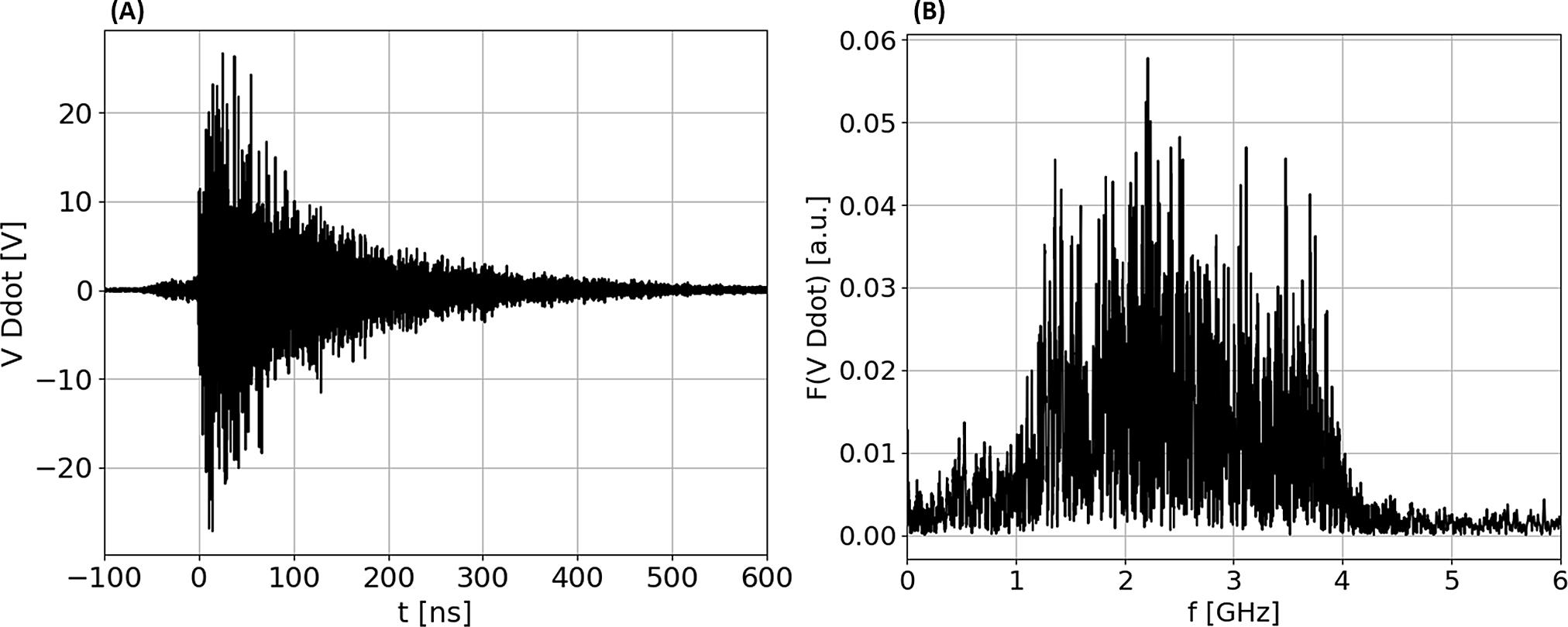

Fig. 2. (a) Time domain signal retrieved by the D-dot probe for shot #32. The timescale has been adjusted in order to overlap t = 0 with the initial rise of the main EMP signal. The small signal at t < 0 is likely due to the laser pre-pulse impinging the target. (b) Frequency domain signal, obtained by the numerical fast Fourier transform of the D-dot time signal. The cut-off at f = 4 GHz is due to the bandwidth limitation of the oscilloscope.

Fig. 3. (a) Electric field () as a function of time, reconstructed from the time signal of the D-dot probe placed between the Teflon and the external chamber wall. The E-fields for shots # 32 (blue plot) and #33 (orange plot) are reported. The laser energy was 19.3 and 21.8 J, respectively. The transient component of the field dominates over the RF oscillations in both cases. (b) The RF component () and the transient component () of shot #32, plotted separately. The signals have been obtained from the signal of panel (a) by applying a low-pass FIR filter (for the transient component) and a high-pass FIR filter (for the RF component).

Fig. 4. (a) Schematic sketch of the charge accumulation effect that occurs on the frontal face of the Teflon. The accelerated protons generate a positive quasi-static charge on the Teflon that, in combination with the chamber wall, acts as a capacitor plate, generating the measured field. (b) Typical proton spectrum obtained during the experimental campaign at from the laser axis, that is, behind the D-dot probe. (c) Top: the temporal evolution of (shot #32) divided into temporal intervals that are associated with the proton populations that were routinely accelerated during the experiment. Below: the TOF signal obtained with the diamond detector placed behind the D-dot. (d) Top: the temporal evolution of (shot #33) divided into temporal intervals that are associated with the proton populations that were routinely accelerated during the experiment. Below: the TOF signal obtained with a diamond detector placed behind the D-dot.

Fig. 5. Comparison between the field, measured during different shots. The field of #31 and #33 (i.e., the shots where the D-dot was rotated) is multiplied by –1 in order to obtain the same field orientation for all shots.

Fig. 6. Schematic view of the particle-in-cell simulations. The simplified model includes the external chamber wall behind the field probe (the orange circle) and the Teflon wall (having dimensions 30 cm × 30 cm × 10 cm, height × width × thickness). The particle emission point (the red circle) is placed at the left-hand limit of the simulation box. The particles propagate from left to right, that is, in the z-direction.

Fig. 7. Comparison between the temporal evolution of the experimental electric field and the simulation results (black line) for shot #32 (a) and shot #33 (b). The timescale of the simulations, similarly as we did for the experimental field, was adjusted in order to superimpose t = 0 and the instant when the electric signal reaches the field probe.

Fig. 8. Field maps of the component, retrieved from the PIC simulation of shots #32 and #33, at the instants t =30 ns ((a) and (d)), ((b) and (e)) and t = 290 ns ((c) and (f)). The x–z plane that we report is the same as the position of the field probe (indicated by the black dot), that is, y = –10 cm, with respect to the height of the particle emission point (at y = 0). The black square indicates the shape of the Teflon.

Table 1. Laser energy, employed target type and EMP electric field characteristics of shots #28, #31, #32 and #33.

Table 2. Particle populations implemented in the PIC simulations of shots #32 and #33. The energy distributions have a uniform spread in all cases.