Development of image invariant moments—a short overview

Kejia Wang; Ziliang Ping; Yunlong Sheng

doi:10.3788/COL201614.091001

Abstract

We give a brief overview on the more than 50 years of development of the moment-based image description, the moment invariants, and the orthogonal moments. Some basic ideas for significantly improving the performance of the image moment-based methods, such as the use of the low-order radial moments for reducing information suppression drawback and the separation of the radial basis from the circular harmonic basis for a free selection of the orthogonal radial polynomials, are presented. Performance measures for the orthogonal moments are discussed from the point of view of image analysis. A moment family list is proposed, which includes most of the representative moments in use and the discrete orthogonal moments.

1. Introduction

Image geometrical moments are region-based integral features useful for describing the image. The moment invariants are combinations of the geometrical moments. They are invariant to scaling, rotation, and other distortions of the image. The orthogonal moments use orthogonal polynomials as the kernel functions in the moment integral. The image moments, moment variants, and orthogonal moments are basic image descriptors and extensively employed for image analysis, shape description, image indexing, annotation, retrieval, registration, matching, object detection, biometric recognition, high level vehicle navigation, image authentication, and image watermarking. Compared with other image descriptors, the moment-based descriptors have rigorous mathematical bases and show the best performance among the low dimensional descriptors for two-dimensional (2D) images^[1].

The first moment invariants have been introduced by Hu^[2] more than half century ago. After a long period of quiet development in the image moment theories, the research on the moment-based methods and their applications found a fast growing period since the 1990s with thousands of journal papers and book chapters published each year in the last ten years. A number of new invariant moments and orthogonal moments have been introduced, showing better performance for image description. In the same time, an important part of the research effort has been devoted to improving the speed and accuracy of the moment feature calculation.

In this Review, we give a short historic overview on the development of the image moment theories involving the moment invariants, the orthogonal moments, and the discrete orthogonal moments. It is impossible to cover the whole area of the image moments in a short overview. Moreover, several excellent textbooks on the image moments theory and applications have been recently published^[3–6]. We describe several selected representative moments, their performance, and the ideas behind their development. We analyze the information suppression drawback in the Zernike moments, which was not addressed in a recent and more complete overview^[7]. We present a moment family table. We also propose new criteria for assessing performance among the numerous orthogonal polynomials. This Review, however, does not cover issues of the computation speed and numerical stability of the image moments nor their applications.

Sign up for Chinese Optics Letters TOC. Get the latest issue of Chinese Optics Letters delivered right to you！Sign up now

2. Moment invariants

The geometrical moments of a 2D image $f (x, y)$ in the rectangular coordinate system are defined as $m_{p, q} = \iint x^{p} y^{q} f (x, y) d x d y,$ (1)where the moment orders $p$ and $q$ are positive integers. Thus, the zero order moment represents the image’s total energy. The first order moments specify the location of the image centroid. The moments computed in the coordinate system with the origin placed at the image centroid are the central moments, which are then translation invariant. The second order moments describe the rectangularity and ellipticity of the image and are used to determine the principle axes of the image^[2,8]. The low-order moment features are directly useful for the shape description in the object detection tasks^[9].

A. Hu’s moment invariants

The moment invariants first introduced by Hu are mostly known as a set of seven parameters, which are invariant to rotation, scaling, and translation of the image^[2]. Hu’s moment invariants are algebraic combinations of the geometrical moments of up to second and third orders obtained by the algebraic invariants theory as $h_{1} = μ_{20} + μ_{02}, h_{2} = {(μ_{20} - μ_{02})}^{2} + 4 μ_{11}^{2}, h_{3} = {(μ_{30} - 3 μ_{12})}^{2} + {(3 μ_{21} - μ_{03})}^{2}, h_{4} = {(μ_{30} + μ_{12})}^{2} + {(μ_{21} + μ_{03})}^{2}, h_{5} = (μ_{30} - 3 μ_{12}) (μ_{30} + μ_{12}) [{(μ_{30} + μ_{12})}^{2} - 3 {(μ_{21} + μ_{03})}^{2}] + (3 μ_{21} - μ_{03}) (μ_{21} + μ_{03}) [3 {(μ_{30} + μ_{12})}^{2} - {(μ_{21} + μ_{03})}^{2}], h_{6} = (μ_{20} - μ_{02}) [{(μ_{30} + μ_{12})}^{2} - {(μ_{21} + μ_{03})}^{2}] + 4 μ_{11} (μ_{30} + μ_{12}) (μ_{21} + μ_{03}), h_{7} = (3 μ_{21} - μ_{03}) (μ_{30} + μ_{12}) [{(μ_{30} + μ_{12})}^{2} - 3 {(μ_{21} + μ_{03})}^{2}] - (μ_{30} - 3 μ_{12}) (μ_{21} + μ_{03}) [3 {(μ_{30} + μ_{12})}^{2} - {(μ_{21} + μ_{03})}^{2}],$ (2)where $μ_{p, q}$ is the central moments. The affine transform invariant moments were also later derived from the algebraic invariant theory^[10]. Hu’s moment invariants are highly concentrated image features and are extensively employed for a long period of time. However, Hu’s moment invariants composed from the low-order geometric moments do not describe the details of the image and suffer from information redundancy and information suppression drawbacks, as first pointed out in Ref. [11]. Hu’s moment invariants are information redundant because the kernels $x^{p} y^{q}$ in their component moments are not orthogonal. As a consequence, an assessment of the quality of the image description by Hu’s moment invariants is not straightforward. One does not know how many Hu’s moment invariants should be used and how well they describe the image for a given task. The information redundancy can be removed by using the orthogonal moments, as will be discussed in Section 3.

B. Fourier-Mellin moments

The information suppression and loss in Hu’s moment invariants may be shown in evidence by the mathematical equivalence between Hu’s moment invariants and the Fourier-Mellin moments. In the polar coordinate system, the Fourier-Mellin moments of an image $f (r, θ)$ are defined as $M_{n, m} = \int_{0}^{2 π} \int_{0}^{1} f (r, θ) r^{n - 1} e^{- j m θ} r d r d θ,$ (3)where the radial coordinate $r$ is normalized for the scale invariance, the positive integer $n \geq 1$ is the radial moment order, and the integer $m$ is the circular harmonic order. A rotation of the image corresponds to a translation of the image along the angular coordinate and a phase shift of the circular Fourier transform, whose intensity is rotation invariant.

In fact, Hu’s moment invariants can be derived more easily in the polar coordinate system as the angular moments^[12] or the Fourier-Mellin moments^[13,14]. It can be shown^[13] that Hu’s moment invariants are equivalent to a special set of the Fourier-Mellin moments with the circular harmonic orders $m = 0 - 3$ and the radial moment order $n = 2$ , 3. It is well known that the low circular harmonic orders $m = 0 - 3$ do not describe angular variations in detail. In general, the circular harmonic orders $m = 0,1, \dots, M$ , up to $M > 10$ are required to reconstruct an image from its circular harmonic functions with acceptable detail^[15]. On the other hand, the high-order monomials $r^{n}$ suppresses contribution to the moments from the central part of the image and heavily weights the contribution of the background outside the object in the image. The information suppression drawback of the moment invariants can be overcame by using the Fourier-Mellin moments of low radial moment orders.

C. Complex moments

The complex moments are defined in the Cartesian coordinate system but with the complex coordinate kernels ( $x + j y$ ) and ( $x - j y$ ) instead of $x$ and $y$ , as in Eq. (1)^[11,16]. The Fourier-Mellin moments in the polar coordinate system are equivalent to the complex moments in the rectangular coordinate system but with some fractional half-integer orders as $M_{n, m} = \int_{0}^{2 π} \int_{0}^{\infty} f (r, θ) r^{n - 1} e^{- j m θ} r d r d θ = \int_{- \infty}^{\infty} \int_{- \infty}^{\infty} f (x, y) {(x + j y)}^{(n - m) / 2} {(x - j y)}^{(n + m) / 2} d x d y,$ (4)so that the Fouirer-Mellin moments can be computed in the rectangular coordinate system via the complex moments without transforming the image from the Cartesian coordinate system to the polar coordinate system. The complex moments were also used to derive the affine invariant moments^[4].

D. Wavelet moments

The wavelet moments are defined in the polar coordinate system as^[17,18] $F_{a, b, m} = \int_{0}^{2 π} \int_{0}^{1} ψ_{a, b} (r) e^{- j m θ} f (r, θ) r d r d θ,$ (5)where the circular Fourier transform gives the rotation invariance, and the wavelet transform is applied in the radial coordinate with the mother wavelets such as the Gabor wavelet, Mexican-hat wavelet, or the cubic B-spline function, the latter is shown as $ψ (r) = \frac{4 α^{n + 1}}{\sqrt{2 π (n + 1)}} σ \cos (2 π f_{0} (2 r - 1)) \exp (- \frac{{(2 r - 1)}^{2}}{2 σ^{2} (n + 1)}),$ (6)where $n = 3$ , $α = 0.697$ , $f_{0} = 0.409$ , and $σ^{2} = 0.561$ . The wavelet transform is a convolution of the image’s circular harmonic function $f_{m} (r) = \int_{0}^{2 π} e^{- j m θ} f (r, θ) d θ,$ (7)with the wavelets, which are scaled, and translated mother wavelets that are shown as $ψ_{a, b} (r) = \frac{1}{\sqrt{a}} ψ (\frac{r - b}{a}),$ (8)where the discrete scaling factor is $a = {(1 / 2)}^{p}$ , the discrete translation factor is $b = (q / 2) {(1 / 2)}^{p}$ , and $p$ and $q$ are positive integers. The continuous wavelets such as the cubic B-spline functions are bandpass filters^[19]. By adaptively choosing the appropriate scale $a$ , the wavelet transform can highlight the local features such as edges in the image. However, the wavelet moments as defined in Eq. (5) are not orthogonal and, therefore, can be used as image features for the image description but not for the image reconstruction. Moreover, the wavelet moments are not scale invariant. The image must be resized to a fixed size before computing the wavelet moments^[17,18].

3. Orthogonal moments

The orthogonal moments are an expansion of the image into the orthogonal polynomial bases. The orthogonal moments are information independent from each other, allowing the image reconstruction for assessing the quality of the image description.

A. Rotation-invariant orthogonal moments

The orthogonal polynomials result from the power series solutions of the ordinary differential equations with the orthogonality of the polynomials related to the Sturm-Liouville forms of the differential equations plus the boundary conditions. They are referred to as the special functions and are given special names because of their frequent uses. On the other hand, the orthogonal polynomials can be easily generated using the Gram-Schmidt orthonormalization, so that there can be an infinite number of orthogonal polynomials. The well-known orthogonal polynomials include the Jacobi, Hermite, Laguerre, and Bessel polynomials. The interrelations between the polynomials exist. For instance, the Gegenbauer, Legendre, Chebyshev, and Zernike polynomials are special cases of the Jacobi polynomials, which are the solutions of the hypergeometric differential equations.

Many orthogonal polynomials are proposed as the bases for the image analysis. For the 2D expansion of an image in the polar coordinate system, the radial orthogonal polynomials are the radial basis, and the Fourier kernels $\exp (j m θ)$ are used for the circular harmonic analysis. As pointed out by Bhatia and Wolf^[20,21], for the rotation invariance in the form, the circular Fourier kernel is a unique solution to be included as the basis function. The scale invariance is achieved by using the normalized radial coordinate.

1. Zernike and Pseudo-Zernike moments

The Zernike moments are orthogonal on the unit circle. The Zernike radial polynomials play a dominant role for the aberration characterization in the optical design. The Zernike moments were proposed in 1980 for image analysis^[22] as $A_{n m} = \frac{n + 1}{π} \int_{0}^{2 π} \int_{0}^{1} R_{n m} (r) \exp (- j m θ) f (r, θ) r d r d θ,$ (9)where the Zernike radial polynomials are $R_{n m} (r) = \sum_{s = 0}^{(n - | m |) / 2} {(- 1)}^{s} \frac{(n - s)!}{s! ((n + | m |) / 2 - s)! ((n - | m |) / 2 - s)!} r^{n - 2 s},$ (10)where $m$ is the circular harmonic order, and $n$ is the degree of the Zernike polynomial. The Zernike moments are designed to be presented in the Cartesian coordinate system, so that the Zernike radial polynomials must not contain powers of $r$ smaller than the circular harmonic order, $n \geq | m |$ and $n - | m |$ are even^[20]. In the Zernike moments, each term of the radial power in $R_{n m} (r)$ corresponds to a radial moment of a specific order, so that the Zernike moments can be computed as the algebraic combinations of the Fourier-Mellin moments.

Bhatia and Wolf derived^[20] another orthogonal set of polynomials in $x$ and $y$ , which contains only the powers of $r$ higher than circular harmonic order $n \geq | m |$ , but with the condition for even $n - | m |$ removed^[20]. This moment set is now referred to as the pseudo-Zernike moments^[23]. When high circular harmonics of the order $m$ are used to represent the image of the angular variation in the range $[0,2 π]$ ^[15], the Zernike and pseudo-Zernike moments with the radial polynomial degrees $n \geq | m |$ must suffer from severe information suppression drawback by the high radial moment orders.

2. Orthogonal Fourier-Mellin moments

The orthogonal Fourier-Mellin moments^[24] are designed to avoid the information suppression issue in the Zernike moments. The orthogonal Fourier-Mellin moments are defined as $Φ_{n m} = \frac{1}{2 π a_{n}} \int_{0}^{2 π} \int_{0}^{1} Q_{n} (r) \exp (- j m θ) f (r, θ) r d r d θ,$ (11)where $a_{n} = ½ (n + 1)$ , and the radial polynomials $Q_{n} (r) = \sum_{s = 0}^{n} α_{n s} r^{s}, with α_{n s} = {(- 1)}^{n + s} \frac{(n + s + 1)!}{(n - s)! s! (s + 1)!} .$ (12)are obtained by the Gram-Schmidt orthogonalization of the power series $r^{n}$ with $n = 0, 1, 2, \dots$ . The orthogonal Fourier-Mellin moments do not need to be expressed in the Cartesian coordinate system. Hence, the restriction of $n \geq | m |$ in the Zernike and pseudo-Zernike moments is removed. This removal of the restriction improves the performance in the image analysis.

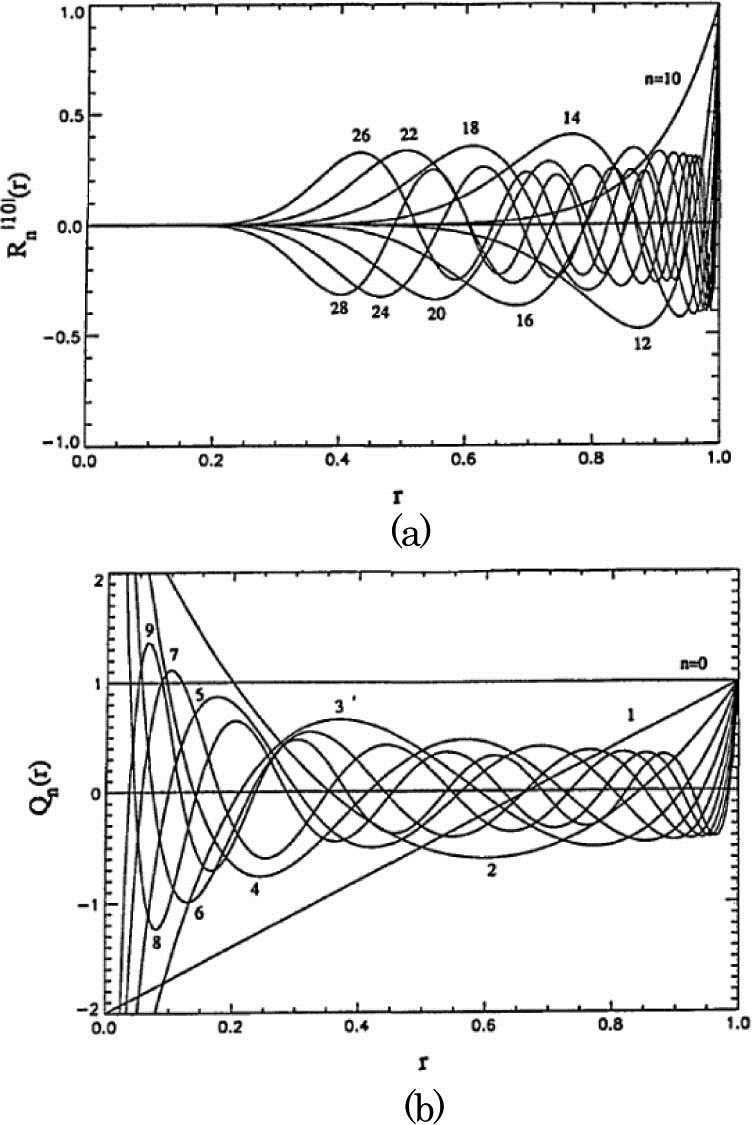
The Fourier-Mellin polynomials $Q_{n} (r)$ have $n$ zeros in $0 \leq r \leq 1$ , while the Zernike polynomials have $(n - m) / 2$ duplicated roots for $R_{n m} (r) = 0$ . To have the same number $n$ of zeros, the degree of the Zernike polynomial must be as high as $2 n + | m |$ . Figure 1 shows the Zernike polynomials $R_{n m} (r)$ for the circular harmonic order $m = 10$ and the degree $n = 10 - 28$ with the zeros distributed in the range of radial distance $r$ $0.2 \leq r \leq 1$ . The closest endpoint to the origin of $R_{28,10} (r)$ is at $r = 0.2$ . The image information in the region of the normalized radial distance $r \leq 0.2$ is then completely suppressed in this set of Zernike moments. The set of orthogonal Fourier-Mellin radial polynomials $Q_{n} (r)$ with the degree $n = 0 - 9$ , independent of $m$ , contain oscillations with the zeros distributed over the radial coordinate range of $0.04 \leq r \leq 1$ , as shown in Fig. 1(b). Thus, the set of orthogonal Fourier-Mellin moments favors the analysis of the image, especially for the central part of the image or the small scale object in the unit circle, which occurs in the context of the scale invariant pattern recognition. Figure 2 shows a capital letter E reconstructed from a maximum of 64 orthogonal Fourier-Mellin moments and those from the Zernike moments. The former in Fig. 2(c) shows much better detail than the latter in Fig. 2(b).

Figure 1.Orthogonal radial polynomials: (a) Zernike polynomials with the degrees $n = 10 - 28$ for circular harmonic order $m = 10$ , (b) orthogonal Fourier-Mellin polynomials with the degrees $n = 0 - 9$ .

Figure 2.(a) Original image of a letter E in the unit disk; (b) reconstructed from first 64 orthogonal Fourier-Mellin moments $Φ_{n, m}$ with $n$ , $m = 0 - 7$ ; (c) reconstructed from Zernike moments $R_{n, m}$ with circular harmonic orders $m = 0 - 7$ and for each $m$ using the eight lowest degrees, satisfying $n \geq | m | + 2$ .

The key idea behind the design of the orthogonal Fourier-Mellin moments is to completely separate the radial polynomials from the circular Fourier kernel, and to avoid the constraint that the radial moment orders should be higher than the circular harmonic orders. Based on this idea, many new orthogonal radial polynomials can be proposed, such as Chebyshev-Fourier, Jacobi-Fourier, and Bessel-Fourier polynomials. All the moments of this type can be computed as algebraic combinations of the Fourier-Mellin moments. The latter can be computed from the equivalent complex moments as shown in Eq. (4) without the transformation of the image from the rectangular to the polar coordinate system.

3. Chebyshev-Fourier moments

The shifted Chebyshev polynomial of the second kind, which is orthogonal in the interval [0,1], is combined with the circular Fourier kernel to form the kernel of the Chebyshev-Fourier moments as^[25] $ϕ_{n m} = \frac{1}{2 π} \int_{0}^{2 π} \int_{0}^{1} R_{n} (r) \exp (- j m θ) f (r, θ) r d r d θ,$ (13)with $n = 0,1, 2 \dots, m = 0, \pm 1, \pm 2, \dots$ and $R_{n} (r) = \sqrt{\frac{8}{π}} {[w (r)]}^{1 / 2} r^{- 1 / 2} U_{n}^{*} (r),$ (14)with shifted Chebyshev polynomials of the second kind $U_{n}^{*} (r) = \sum_{k = 0}^{[n / 2]} {(- 1)}^{k} \frac{(n - k)!}{k! (n - 2 k)!} {[2 (2 r - 1)]}^{n - 2 k},$ (15)which are orthogonal over the range $0 \leq r \leq 1$ as $\int_{0}^{1} U_{n}^{*} (r) U_{k}^{*} (r) w (r) d r = \frac{π}{8} δ_{n k},$ (16)where $δ_{n k}$ is the Kronecker symbol, and $w (r) = {(r - r^{2})}^{1 / 2}$ is the weight function. As shown in Fig. 3, $R_{n} (r)$ possesses $n$ zero points evenly distributed over the interval [0,1]. The oscillation amplitude of the $R_{n} (r)$ of various degrees $n$ are close to constant in a large portion of the radial interval [0,1], except that when $r$ tends to be zero, $R_{n} (r)$ tends to be high absolute values, as shown in Fig. 3. This can be a potential drawback. Experiments showed^[25] that the performance for describing an image of the Chebyshev-Fourier moments is similar as that of the orthogonal Fourier-Mellin moments^[25].

Figure 3.Shifted Chebyshev polynomial $R_{n (r)}$ with $n = 1$ , 2, 9, 10, [25]

4. Generic Jacobi-Fourier moments

The Jacobi-Fourier moments are referred to as the generic orthogonal moments^[26] with the kernel composed of the radial Jacobi polynomial and the angular Fourier complex exponential kernel, and are defined as $Φ_{n m} = \frac{1}{2 π} \int_{0}^{2 π} \int_{0}^{1} J_{n} (p, q, r) \exp (- j m θ) f (r, θ) r d r d θ,$ (17)where the radial Jacobi polynomials are generated by the orthogonalization of the natural power sequence of the radial coordinate with the weighting function^[20,27] as $w (p, q, r) = {(1 - r)}^{p - q} r^{q - 1},$ (18)where $p - q > - 1, q > 0$ , such as $\int_{0}^{1} G_{n} (p, q, r) G_{k} (p, q, r) w (p, q, r) d r = b_{n} (p, q) δ_{n k},$ (19)and the radial Jacobi polynomials are $G_{n} (p, q, r) = \frac{n! Γ (q)}{Γ (n + p)} \sum_{s = 0}^{n} {(- 1)}^{n - s} \frac{Γ (n + p + s)}{(n - s)! s! Γ (q + s)} r^{s},$ (20)which become, after the normalization, $J_{n} (p, q, r) = G_{n} (p, q, r) \sqrt{w (p, q, r) / b_{n} (p, q, r)} .$ (21)where the normalization constant is $b_{n} (p, q) = \frac{n! Γ (n + p - q + 1) {[Γ (q)]}^{2}}{(2 n + p) Γ (n + p) Γ (n + q)} .$ (22)It can be shown that the Jacobi-Fourier moment corresponds to the Legendre-Fourier moments with $p = q = 1$ and the unit weighting function, the Chebyshev-Fourier moments with $p = 2$ and $q = 3 / 2$ , and the orthogonal Fourier-Mellin moments with $p = q = 2$ and the weighting function equal to $r$ ^[26]. The Zernike radial polynomial corresponds to the Jacobi radial polynomial as $r^{m} J_{k} (p, q, r^{2})$ with $p = q = m + 1$ , where $m$ is the circular harmonic order in the Zernike moments, and $k = (n - m) / 2$ . The pseudo-Zernike radial polynomial corresponds to the Jacobi radial polynomial $J_{k} (p, q, r)$ with $p = 2 m + 2$ , $q = m + 2$ and $k = n - m$ ^[3]. Therefore, the Jacobi-Fourier moments provide a generic framework to express the rotation-invariant orthogonal moments. The common formulation is a benefit for the performance comparison and analysis of the orthogonal moments and for searching prime orthogonal moments.

5. Bessel-Fourier moments

The Bessel-Fourier moments were introduced recently, which are defined as^[28] $B_{n m} = \frac{1}{2 π α_{n}} \int_{0}^{2 π} \int_{0}^{1} J_{v} (λ_{n} r) \exp (- j m θ) f (r, θ) r d r d θ,$ (23)where $J_{v} (λ_{n} r)$ is the Bessel radial polynomials of order $v$ of the first kind, and $λ_{n}$ is the $n$ th zero of $J_{v} (λ_{n}) = 0$ . The Bessel polynomials of the same order $v$ are orthogonal over the radial interval [0,1], such as $\int_{0}^{1} J_{v} (λ_{n} r) J_{v} (λ_{k} r) d r = α_{n} δ_{n k},$ (24)where $α_{n} = {[J_{v + 1} (λ_{n})]}^{2} / 2$ is the normalization constant. Figure 4 is a plot of the Bessel function $v = 1$ . The Bessel polynomials of the first kind $J_{1} (λ_{n} r)$ tend to be zero at both ends of the radial interval [0,1] and show a slow variation of the oscillation amplitude over the radial range [0,1], as shown in Fig. 4. Only in the range of $r$ close to $r = 0$ , the oscillation amplitudes are doubled.

Figure 4.Bessel Radial polynomial $J_{1}$ ( $λ_{n} r$ ) with $n = 0,1, \dots, 9$ , [28].

Compared to the orthogonal Fourier-Mellin polynomials and the shifted Chebyshev polynomials, both of which tend to have high values when $r$ tends to be zero, as shown in Figs. 1 and 3, the Bessel-Fourier moments show a better performance for image analysis. They also are better than the Zernike moments, as the Zernike moments show a sharp increase to the unit when $r$ tends to be $r = 1$ , as shown in Fig. 1(a).

6. Radial-Harmonic-Fourier transform

The radial-harmonic-Fourier moments^[29], or polar harmonic transform^[30,31], includes the Fourier harmonic analysis in both the radial and angular coordinates and are defined as $ϕ_{n m} = \frac{1}{2 π} \int_{0}^{2 π} \int_{0}^{1} T_{n} (r) \exp (- j m θ) f (r, θ) r d r d θ .$ (25)where the radial kernels $T_{n} (r)$ are the orthogonal triangular functions, such as $T_{n} (r) = \sin [(n + 1) π r$ ] for the odd $n$ , and $T_{n} (r) = \cos (n π r)$ for the even $n$ , or the complex exponential functions such as $T_{n} (r) = \exp (j 2 π n r^{2})$ or $T_{n} (r) = \exp (j n r)$ . In all cases, the $T_{n} (r)$ should be normalized, respectively. The corresponding transforms are referred to as the radial-harmonic-Fourier moments^[29], the polar harmonic transform^[30], and the exponent-Fourier moments^[31]. The angular radial transform, the polar complex exponential transform, the polar cosine transform, and the polar sine transform also belong to this group^[31–33]. As the Fourier kernels have uniform distributions of the zeros and a constant oscillation amplitude over the interval $0 \leq r \leq 1$ and $0 \leq θ \leq 2 π$ , this type of transform shows a superior performance over the other rotation-invariant orthogonal moments with radial polynomial kernels^[34].

The radial-harmonic-Fourier moments are not scale invariant. An image must be rescaled to a given size before computing the moments. Moreover, the radial-harmonic-Fourier moments should preferably be referred to as the radial-harmonic-Fourier transforms, as the moments are essentially formulated with the monomial and polynomial kernels. Moreover, the moments with the radial polynomials can achieve the scale invariance by using the normalized radial coordinate.

B. Orthogonal moments in the Cartesian coordinate system

There are an infinite number of complete sets of orthogonal polynomials. Many of them were proposed as the kernels of the orthogonal moments for 2D images in the Cartesian coordinate system. The orthogonal moments in this category include the Legendre moments^[22,35], the Gegenbauer moments^[36,37], the Gaussian-Hermite moments^[38–40], etc. Defined in the Cartesian coordinate system, these moments enjoy the orthogonality of the orthogonal polynomials in $x$ and $y$ in the interval $[- 1,1]$ or [0,1] for image analysis and reconstruction. They can also be scale invariant when using the scaling factor to normalize the coordinates.

A new type of the orthogonal moments uses two different polynomials as the basis for each dimension in the Cartesian coordinate system separately, such as the Chebyshev-Gegenbauer and the Gegenbauer-Legendre moments. These moments are called separable moments^[41,42].

The orthogonal moments in the Cartesian coordinate system are not rotational invariant by definition. However, the rotation invariance can still be introduced by the transformation between the Cartesian and polar coordinate systems.

C. Performance measures of orthogonal moments

Performances of the orthogonal moment image descriptors have been assessed in many Letters via the image reconstruction errors and the pattern recognition scores. However, these merits are dependent on the selected moment orders and the testing image, and therefore are the indirect measures. In fact, as the orthogonal moments are the expansions of the image into the orthogonal polynomial bases, the performance of the image description by the orthogonal moments is determined directly by the bases’ functions. In the case of rotation-invariant orthogonal moments, the Fourier harmonic analysis is applied along the angular coordinate. Hence, the performance of the image analysis along the radial coordinate depends uniquely on the set of the radial orthogonal polynomials. For the image analysis, the radial polynomial set should have a high number of real-valued zeros, a wide range of the distribution of zeros in the whole range $0 \leq r \leq 1$ , and a constant oscillation amplitude. From instance, the Zernike radial polynomials are restricted to having high degrees, and one set of Zernike moments, shown in Fig. 1(a), have the zeros distributed in the range of $0.2 \leq r \leq 1$ . The orthogonal Fourier-Mellin polynomials and shifted Chebyshev polynomials both tend to have high values when $r$ tends to be zero, as shown in Figs. 1(b) and 3. Those facts represent the weakness of these moments. The Bessel polynomials have $n + 2$ zeros distributed in the range of $0 \leq r \leq 1$ , and a slow variation of the oscillation amplitudes, as shown in Fig. 4, so that they can have a better performance for the image analysis. In this sense, the radial-harmonic-Fourier transforms have the best performance, as this is simply the Fourier harmonic analysis in both the angular and radial dimensions. However, they are not image moments in the mathematical sense and are not scale invariant.

Furthermore, in terms of the space-frequency space analysis, the Fourier kernels, which are perfectly local in frequency but are global in space, are not efficient for describing local details in the image. The Fourier moments miss the location of an image detail, and very high frequency orders must be involved to reconstruct a sharp detail, such as an edge in the image. In this sense, the wavelet moment using the Gabor transform and the wavelet transform can be superior over the Fourier transform^[43]. However, the wavelet moments using the continuous mother wavelets are not orthogonal.

Table 1 shows a family of the moments with the classification. However, it is regrettable to not be able to list all image moments in Table 1 in the period of time when many novel moments are being proposed. For a given image description task, the choice among the available moments should depend on the specific tasks, the requested invariance, the computation performance, and many other considerations.

D. Discrete orthogonal moments

Most orthogonal moments discussed previously belong to continuous moments, as their bases are continuous functions with their orthogonality defined by the continuous integrals. Numerical computation of the continuous moments requires discretization of the continuous polynomials and discrete approximation of the continuous moment integrals, which causes the errors, affecting the accuracy of the calculation and the quality of image reconstruction with increased computational complexity.

Non-orthogonal moments	Moment invariants (Hu’s) Fourier-Mellin moments complex moments wavelet moments
Orthogonal moments	Continuous orthogonal moments	Cartesian moments	Legendre moments Gaussian-Hermite moments Gegenbauer moments
	Continuous orthogonal moments	Circular moments	Zernike moments pseudo-Zernike moments orthogonal Fourier-Mellin moments Chebyshev-Fourier moments Jacobi-Fourier moments Bessel-Fourier moments radial-harmonic-Fourier transform
	Discrete orthogonal moments	Cartesian moments	Tchebichef moments Krawtchouk moments Hahn moments dual Hahn moments Racah moments
	Discrete orthogonal moments	Circular moments	Radial Tchebichef moments radial Krawtchouk moments

Table 1. Family of Image Moments

View all Tables

The discrete orthogonal moments^[44–55] use discrete orthogonal polynomials as the basis set, which satisfies the orthogonality exactly without numerical approximation. For a smooth image intensity distribution, whose value is known only at a set of discrete coordinate points, the discrete polynomials $p_{n} (x)$ are also defined on these distinct real nodes, and satisfy the discrete orthogonality relation as $\sum_{x = 0}^{N - 1} p_{m} (x) p_{n} (x) w (x) = ρ (n) δ_{m n},$ (26)where $0 \leq m, n \leq N - 1$ , and $ρ (n)$ is the square norm of $p_{n} (x)$ . The weight $w (x)$ in the orthogonality expression (26) of the discrete polynomials can be the Meixner, Charlier, Krawtchouk, and Hahn weight. Thus, the discrete orthogonal polynomials are uniquely determined by the given distinct nodes support, the weights, and the orthogonality condition, and can be built from monomials by the Gram-Schmidt process.

The discrete orthogonal moments of a 2D image $f (x, y)$ in the Cartesian coordinate system on a closed interval are defined as $P_{m n} = \sum_{x = 0}^{M - 1} \sum_{y = 0}^{N - 1} f (x, y) {\tilde{p}}_{m} (x) {\tilde{p}}_{n} (y),$ (27)where the normalized discrete polynomial bases ${\tilde{p}}_{n} (x)$ are shown as ${\tilde{p}}_{n} (x) = p_{n} (x) \sqrt{w (x) / ρ (n)} .$ (28)As the discrete polynomials satisfy the orthogonal property precisely, no approximation errors are involved in the computation of moments. The image can be accurately reconstructed from the complete set of discrete moments. When two different discrete orthogonal polynomials serve as the bases in $x$ and $y$ , separately, the moments are separable moments such as that using the Tchebichef-Krawtchouk, Hahn-Krawtchouk, and Charlier-Hahn polynomials combined with Tchebichef, Krawtchouk, Hahn, or Charlier polynomials^[41,42].

1. Discrete orthogonal Tchebichef moments

The first discrete orthogonal Tchebichef (Chebyshev) moments^[44] were proposed based on the discrete orthogonal Tchebichef polynomials. The discrete Tchebichef polynomials are shown as $t_{n} (x) = n! \sum_{k = 0}^{n} {(- 1)}^{n - k} (\begin{array}{l} N - 1 - k \\ n - k \end{array}) (\begin{array}{l} n + k \\ n \end{array}) (\begin{array}{l} x \\ k \end{array}),$ (29)satisfying the orthogonality condition with the unit weight and the normalization constants $ρ (n, N) = \frac{N (N^{2} - 1) (N^{2} - 2^{2}) \dots (N^{2} - n^{2})}{2 n + 1} = (2 n)! (\begin{matrix} N + n \\ 2 n + 1 \end{matrix}), n = 0,1, \dots N - 1 .$ (30)The normalized Tchebichef polynomials are ${\tilde{t}}_{n} (x) = t_{n} (x) / β (n, N),$ (31)with the normalized constant $\tilde{ρ} (n, N) = ρ (n, N) / β {(n, N)}^{2} and β (n, N) = N^{n} .$ (32)The discrete Tchebichef moments exhibit a superior performance for image reconstruction and feature representation compared to the continuous Legendre and Zernike moments^[44].

2. Discrete orthogonal Krawtchouk moments

One of representative discrete orthogonal moments defined in the Cartesian coordinate system is the Krawtchouk^[46] moment, which are based on the Krawtchouk polynomials. The kernel functions are the separable discrete orthogonal polynomials in $x$ and $y$ . The discrete Krawtchouk polynomials satisfy the orthogonality conditions with the Krawtchouk weight as $w (x; p, N) = (\begin{array}{l} N \\ x \end{array}) p^{x} {(1 - p)}^{N - x},$ (33)and the normalization constant $ρ (n; p, N) = {(- 1)}^{n} {(\frac{1 - p}{p})}^{n} \frac{n!}{{(- N)}_{n}} .$ (34)The Krawtchouk polynomials are obtained as $K_{n} (x; p, N) = \sum_{k = 0}^{N} a_{k, n, p} x^{k} = {}_{2}F_{1} (- n, - x; - N; \frac{1}{p}),$ (35)where $x, n = 0,1, 2 \dots, N$ , $N > 0$ , and $p \in (0,1)$ , the ${{}_{r}F}_{s}$ is the hypergeometric series, defined as ${{}_{r}F}_{s} (a_{1}, \dots, a_{r}; b_{1}, \dots, b_{s}; z) = \sum_{k = 0}^{\infty} \frac{{(a_{1})}_{k} {(a_{2})}_{k} \dots {(a_{r})}_{k}}{{(b_{1})}_{k} {(b_{1})}_{k} \dots {(b_{s})}_{k}} \frac{z^{k}}{k!},$ (36)and ${(a)}_{k}$ is the Pochhammer symbol given by ${(a)}_{k} = a (a + 1) \dots (a + k - 1) = \frac{Γ (a + k)}{Γ (a)} .$ (37)The Krawtchouk moments perform better than the Tchebichef moments in terms of the reconstruction error. They were employed to extract local features of an image by varying the parameter of the binomial distribution associated with the Krawtchouk polynomials^[46].

3. Discrete orthogonal Hahn moments

Two types of Hahn polynomials with different standardizations were used to define two types of Hahn moments^[47,48], respectively. The Hahn polynomials are expressed as $h_{n}^{(μ, ν)} (x, N) = {(N + ν - 1)}_{n} {(N - 1)}_{n} \times \sum_{k = 0}^{n} {(- 1)}^{k} \frac{{(- n)}_{k} {(- x)}_{k} {(2 N + μ + ν - n - 1)}_{k}}{{(N + ν - 1)}_{k} {(N - 1)}_{k}} \frac{1}{k!},$ (38)where $μ, ν (μ > - 1, ν > - 1)$ are the adjustable parameters controlling the shape of the polynomials. The Hahn polynomials satisfy the discrete orthogonal condition as $\sum_{x = 0}^{N - 1} w (x) h_{m}^{(μ, ν)} (x, N) h_{n}^{(μ, ν)} (x, N) = d_{n}^{2} δ_{m n},$ (39)with the weighting function as $w (x) = \frac{1}{Γ (x + 1) Γ (x + μ + 1) Γ (N + ν - x) Γ (N - n - x)},$ (40)and the square norm $d_{n}^{2}$ has the following expression $d_{n}^{2} = \frac{Γ (2 N + μ + ν - n)}{(2 N + μ + ν - 2 n - 1) Γ (N + μ + ν - n)} \times \frac{1}{Γ (N + μ - n) Γ (N + ν - n) Γ (n + 1) Γ (N - n)} .$ (41)Compared with the Tchebichef moments and the Krawtchouk moments, the first type of Hahn moments has better image reconstruction results^[47]. Another type of Hahn moments^[48] is based on another form of Hahn polynomials, shown as $h_{n} (x; α, β, N) = {}_{3}F_{2} (- n, n + α + β + 1, - x; α + 1, - N; 1),$ (42)where $x, n = 0,1, 2, \dots, N - 1$ , $α > - 1, β > - 1$ , or $α < - N$ , $β < - N$ , with the weighting function $w (x; α, β, N) = (\begin{matrix} α + x \\ x \end{matrix}) (\begin{matrix} β + N - x \\ N - x \end{matrix}),$ (43)and the square norm $d^{2} (n; α, β, N) = \frac{{(- 1)}^{n} {(n + α + β + 1)}_{N + 1} {(β + 1)}_{n} n!}{(2 n + α + β + 1) {(α + 1)}_{n} {(- N)}_{n} N!} .$ (44)This type of Hahn moments provides a unified understanding of the Tchebichef and Krawtchouk moments. The two latter moments can be obtained as particular cases of the Hahn moments with the appropriate parameter settings. This fact implies that the Hahn moments encompass all their properties and exhibit intermediate properties between the extremes set by the Tchebichef and Krawtchouk moments. Besides, the Hahn moments, as a generalization of the Tchebichef and Krawtchouk moments, can be used for global and local feature extraction^[48].

4. Discrete orthogonal dual Hahn moments

The discrete Tchebichef, Krawtchouk, and Hahn polynomials are orthogonal on a uniform lattice ${x = 0,1, 2, \dots}$ . There is another category of discrete variable polynomials, which are orthogonal on a non-uniform lattice ${x = x (s), s = 0,1, 2, \dots}$ . For different non-uniform lattice functions, there are different polynomials. The dual Hahn polynomials and the Racah polynomials are two types of discrete polynomials orthogonal on a non-uniform lattice $x (s) = s (s + 1)$ . Due to the finite domain of the definition, the dual Hahn polynomials and Racah polynomials were explored to construct the corresponding dual Hahn moments^[50] and Racah moments^[52]. They are defined in the Cartesian coordinate system, and their kernel functions are the product of two corresponding two corresponding 1D separable discrete orthogonal polynomials.

Given a uniform pixel lattice image $f (s, t)$ with a size $N \times N$ , the dual Hahn moments^[50] are defined as $W_{n m} = \sum_{s = a}^{b - 1} \sum_{t = a}^{b - 1} {\hat{w}}_{n}^{(c)} (s, a, b) {\hat{w}}_{m}^{(c)} (t, a, b) f (s, t),$ (45)with $n, m = 0,1, 2, \dots, N - 1$ , and the dual Hahn polynomials $w_{n}^{(c)} (s, a, b)$ defined as $w_{n}^{(c)} (s, a, b) = \frac{{(a - b + 1)}_{n} {(a + c + 1)}_{n}}{n!} \times {}_{3}F_{2} (- n, a - s, a + s + 1; a - b + 1, a + c + 1; 1),$ (46)where parameters $a$ , $b$ , and $c$ are restricted to $- (1 / 2) < a < b$ , $| c | < 1 + a, b = a + N$ . The dual Hahn polynomials satisfy the following orthogonality property $\sum_{s = a}^{b - 1} ρ (s) w_{n}^{(c)} (s, a, b) w_{m}^{(c)} (s, a, b) [Δ x (s - \frac{1}{2})] = d_{n}^{2} δ_{n m} .$ (47)where $ρ (s)$ is the weighting function $ρ (s) = \frac{Γ (a + s + 1) Γ (c + s + 1)}{Γ (s - a + 1) Γ (b - s) Γ (b + s + 1) Γ (s - c + 1)},$ (48)and $d_{n}^{2}$ is the square norm $d_{n}^{2} = \frac{Γ (a + c + n + 1)}{n! (b - a - n - 1)! Γ (b - c - n)} .$ (49)The normalized dual Hahn polynomials are ${\hat{w}}_{n}^{(c)} (s, a, b) = w_{n}^{(c)} (s, a, b) \sqrt{\frac{ρ (s)}{d_{n}^{2}} [Δ x (s - \frac{1}{2})]} .$ (50)The Tchebichef polynomials, Krawtchouk polynomials, and Hahn polynomials are special cases of the dual Hahn polynomials. Thus, the dual Hahn moments which contain more parameters have a generality and give more flexibility to promote the image describing ability. The dual Hahn moments perform better than the Legendre moments, Tchebichef moments, and Krawtchouk moments in terms of image reconstruction capability^[50].

5. Discrete orthogonal Racah moments

Similar to the dual Hahn moments, for the image $f (s, t)$ with a size $N \times N$ , the Racah moments^[52] are defined as $U_{n m} = \sum_{s = a}^{b - 1} \sum_{t = a}^{b - 1} {\hat{u}}_{n}^{(α, β)} (s, a, b) {\hat{u}}_{m}^{(α, β)} (t, a, b) f (s, t),$ (51)with $n, m = 0,1, 2, \dots, N - 1$ . Racah polynomials $u_{n}^{(α, β)} (s, a, b)$ are defined as $u_{n}^{(α, β)} (s, a, b) = \frac{1}{n!} {(a - b + 1)}_{n} {(β + 1)}_{n} {(a + b + α + 1)}_{n} \times {}_{4}F_{3} (- n, α + β + n + 1, a - s, a + s + 1; β + 1, a - b + 1, a + b + α + 1; 1),$ (52)where the parameters $a, b, α$ and $β$ are restricted by $- (1 / 2) < a < b, α > - 1, - 1 < β < 2 a + 1, b = a + N .$ The Racah polynomials satisfy the following orthogonality property $\sum_{s = a}^{b - 1} ρ (s) u_{n}^{(α, β)} (s, a, b) u_{m}^{(α, β)} (s, a, b) [Δ x (s - \frac{1}{2})] = d_{n}^{2} δ_{n m},$ (53)with the weight $ρ (s) = \frac{Γ (a + s + 1) Γ (s - a + β + 1) Γ (b + α - s) Γ (b + α + s + 1)}{Γ (a - β + s + 1) Γ (s - a + 1) Γ (b - s) Γ (b + s + 1)},$ (54)and the square norm $d_{n}^{2} = \frac{Γ (α + n + 1) Γ (β + n + 1) Γ (b - a + α + β + n + 1)}{(α + β + 2 n + 1) n! (b - a - n - 1)! Γ (α + β + n + 1)} \times \frac{Γ (a + b + α + n + 1)}{Γ (a + b - β - n)} .$ (55)The normalized Racah polynomials are ${\hat{u}}_{n}^{(α, β)} (s, a, b) = u_{n}^{(α, β)} (s, a, b) \sqrt{\frac{ρ (s)}{d_{n}^{2}} [Δ x (s - \frac{1}{2})]} .$ (56)The Racah moments perform better than the Legendre moments, Tchebichef moments, and Krawtchouk moments for noise-free image reconstruction^[52].

6. Rotation-invariant discrete orthogonal moments

Rotation-invariant discrete radial Tchebichef moments defined in polar coordinate systems were proposed based on the 1D radial discrete Tchebichef polynomials and the circular Fourier kernel^[53]. The primary advantage of the discrete radial moments is the rotational invariance. For an image $f (r, θ_{k})$ , the explicit expressions of the radial Tchebichef moments^[53] are as follows: $S_{p q} = \frac{1}{n ρ (p, m)} \sum_{r = 0}^{m - 1} \sum_{k = 0}^{n - 1} t_{p, m} (r) e^{- j \frac{2 π q k}{n}} f (r, θ_{k}),$ (57)where $r = 0,1, \dots, m - 1$ , $m = N / 2, θ_{k} = 2 π k / n$ , and $k = 0,1, \dots, n - 1$ , with $n$ denoting the maximum number of pixels along the circumference of the circle of radius $m$ , $t_{p, m} (r) = \frac{p!}{m^{p}} \sum_{k = 0}^{p} {(- 1)}^{p - k} (\begin{array}{l} m - 1 - k \\ p - k \end{array}) (\begin{array}{l} p + k \\ p \end{array}) (\begin{array}{l} r \\ k \end{array}),$ (58) $ρ (p, m) = \frac{m (1 - \frac{1}{m^{2}}) (1 - \frac{2^{2}}{m^{2}}) \dots (1 - \frac{p^{2}}{m^{2}})}{2 p + 1},$ (59)with $p = 0,1, \dots m - 1$ . The rotation-invariant discrete radial Krawtchouk moments^[54] were introduced in a similar way to the radial Tchebichef moments. The kernel functions of the radial Krawtchouk moments are products of radial 1D Krawtchouk polynomials and angular circular Fourier functions.

4. Conclusion

We have reviewed some major steps in the development of the image moment theory, involving the geometrical moments, the moment invariants, and the orthogonal moments. It is impossible for this short Review to cover all the important moments in detail. Moreover, we have not included in this Review the works on the speed and accuracy of computation of the image moments and on their applications. A large body of excellent Letters and text books exist in the literature now. A more rigorous, accurate, and complete mathematical analysis on the image moments theory has been developed. However, some fundamental intuitive ideas, such as the use of low-order radial moments for avoiding information suppression, the definition of the moment invariants in the polar coordinate system and relation of them to the moments in the rectangular coordinate system via the complex moments, and the separation of the radial moment orders from the circular harmonic orders, have been widely accepted and continuously used in the development of the image moment-based methods. We proposed a moment family table and the performance measures for the orthogonal moments based on the number of zeros, the uniform distribution of zeros, and the oscillation amplitude variation of the orthogonal polynomials. The image reconstruction can depend on the choice of moment orders and on the testing image set so that they can be indirect measures for the performance.

References

[1] K. Mikolajczyk, C. Schmid. IEEE Trans. Pattern Anal. Mach. Intell., 27, 1615(2005).

[2] M. K. Hu. IRE Trans. Inform. Theor., IT-8, 179(1962).

[3] G. A. Papakostas. Moments and Moment Invariants—Theory and Applications(2014).

[4] J. Flusser, T. Suk, B. Zitová. Moments and Moment Invariants in Pattern Recognition(2009).

[5] R. Mukundan, K. Ramakrishnan. Moment Functions in Image Analysis—Theory and Applications(1998).

[6] M. Pawlak. Image Analysis by Moments: Reconstruction and Computational Aspects(2006).

[7] G. A. Papakostas. Over 50 Years of Image Moments and Moment Invariants(2014).

[8] Y. Sheng, H. Arsenault. J. Opt. Soc. Am. A, 4, 1176(1987).

[9] S. A. Dudani, K. J. Breeding. IEEE Trans. Comput., c-26, 39(1977).

[10] J. Flusser, T. Suk. Pattern. Recognit., 26, 167(1993).

[11] Y. S. Abu-Mostafa, D. Psaltis. IEEE Trans. Pattern Anal. Mach. Intell., PAMI-6, 698(1984).

[12] J. F. Boyce, W. J. Hossack. Pattern. Recognit. Lett., 1, 451(1983).

[13] Y. Sheng, J. Duvernoy. J. Opt. Soc. Am. A, 3, 885(1986).

[14] Y. Sheng, H. H. Arsenault. J. Opt. Soc. Am. A, 3, 771(1986).

[15] H. H. Arsenault, Y. Sheng. Appl. Opt., 25, 3225(1986).

[16] Y. S. Abu-Mostafa, D. Psaltis. IEEE Trans. Pattern Anal. Mach. Intell., PAMI-7, 46(1985).

[17] D. Shen, H. H. Ip. Pattern Recognit., 32, 151(1999).

[18] X. Hu, B. Kong, F. Zheng, S. Wang. International Conference on Information Acquisition(2007).

[19] H. Szu, Y. Sheng, J. Chen. Appl. Opt., 31, 3267(1992).

[20] A. B. Bhatia, E. Wolf. Mathematical Proceedings of the Cambridge Philosophical Society, 50, 40(1954).

[21] M. Born, E. Wolf. Principles of Optics(1975).

[22] M. R. Teague. J. Opt. Soc. Am., 70, 920(1980).

[23] C. H. Teh, R. T. Chin. IEEE Trans. Pattern Anal. Mach. Intell., 10, 496(1988).

[24] Y. Sheng, L. Shen. J. Opt. Soc. Am. A, 11, 1748(1994).

[25] Z. Ping, R. Wu, Y. Sheng. J. Opt. Soc. Am. A, 19, 1748(2002).

[26] Z. L. Ping, H. P. Ren, J. Zou, Y. L. Sheng, W. Bo. Pattern. Recognit., 40, 1245(2007).

[27] M. Abramowitz, I. A. Stegun. Handbook of Mathematical Functions: With Formulas, Graphs, and Mathematical Tables(1964).

[28] B. Xiao, J.-F. Ma, X. Wang. Pattern. Recognit., 43, 2620(2010).

[29] H. Ren, Z. Ping, W. Bo, W. Wu, Y. Sheng. J. Opt. Soc. Am. A, 20, 631(2003).

[30] P. Yap, X. Jiang, A. C. Kot. IEEE Trans. Pattern Anal. Mach. Intell., 32, 1259(2010).

[31] T. V. Hoang, S. Tabbone. Proceedings of 18th IEEE International Conference on Image Processing (ICIP), 829(2011).

[32] H. T. Hu, Y. D. Zhang, C. Shao, Q. Ju. Pattern Recognit., 47, 2596(2014).

[33] Q. Miao, J. Liu, W. Li, J. Shi, Y. Wang. Opt. Commun., 285, 1044(2012).

[34] M. Bober. IEEE Trans. Circ. Syst. Video Tech., 11, 716(2001).

[35] C.-W. Chong, P. Raveendran, R. Mukundan. Pattern. Recognit., 37, 119(2004).

[36] S. Liao, A. Chiang, L. Qin, M. Pawlak. Proceedings of 16th International Conference on Pattern Recognition, 485(2002).

[37] K. M. Hosny. Pattern. Recognit. Lett., 32, 795(2011).

[38] B. Yang, M. Dai. Signal Process., 91, 2290(2011).

[39] B. Yang, G. Li, H. Zhang, M. Dai. Pattern. Recognit. Lett., 32, 1283(2011).

[40] L. Geng-Xiang, Y. Bo, D. Mo. Proceedings of International Conference on Wavelet Analysis and Pattern Recognition (ICWAPR), 12(2011).

[41] A. Hmimid, M. Sayyouri, H. Qjidaa. J. Electron. Imaging, 23, 013026(2014).

[42] H. Zhu. Pattern Recognit., 45, 1540(2010).

[43] Y. Sheng. Wavelet transform. Transforms and Applications(2010).

[44] R. Mukundan, S. H. Ong, P. A. Lee. IEEE Trans. Image Process., 10, 1357(2001).

[45] H. Zhu, H. Shu, T. Xia, L. Luo, J. Louis Coatrieux. Pattern. Recognit., 40, 2530(2007).

[46] P. T. Yap, R. Paramesran, O. Seng-Huat. IEEE Trans. Image Process., 12, 1367(2003).

[47] M. Kamel, J. Zhou, H. Shu, A. Campilho, H. Zhu, C. Toumoulin, L. Luo. Image Analysis and Recognition, 524(2005).

[48] Y. Pew-Thian, R. Paramesran, O. Seng-Huat. IEEE Trans. Pattern Anal. Mach. Intell., 29, 2057(2007).

[49] H.-A. Goh, C.-W. Chong, R. Besar, F. S. Abas, K.-S. Sim. Int. J. Image Graph., 9, 271(2009).

[50] H. Zhu, H. Shu, J. Zhou, L. Luo, J. L. Coatrieux. Pattern. Recognit. Lett., 28, 1688(2007).

[51] E. G. Karakasis, G. A. Papakostas, D. E. Koulouriotis, V. D. Tourassis. Pattern. Recognit., 46, 1998(2013).

[52] H. Zhu, H. Shu, J. Liang, L. Luo, J.-L. Coatrieux. Signal Process., 87, 687(2007).

[53] R. Mukundan. TENCON: 2005 IEEE Region 10, 1(2005).

[54] P. Ananth raj, A. Venkataramana. Proceedings of 6th International Conference on Information, Communications & Signal, 1(2007).

[55] H. Zhu, M. Liu, H. Shu, H. Zhang, L. Luo. IET Image Process., 4, 335(2010).