
Kevin van As, Bram A. Simons, Chris R. Kleijn, Sasa Kenjeres, Nandini Bhattacharya. The dependence of speckle contrast on velocity: a numerical study[J]. Journal of the European Optical Society-Rapid Publications, 2022, 18(2): 2022010
Journals >Journal of the European Optical Society-Rapid Publications >Volume 18 >Issue 2 >Page 2022010 > Article
- Journal of the European Optical Society-Rapid Publications
- Vol. 18, Issue 2, 2022010 (2022)
Abstract
1 Introduction
Laser speckle contrast imaging (LSCI) is a promising technique for the non-invasive measurement of dynamic systems (i.e., flowmetry), such as blood flow [
However, quantitative measurements with LSCI have been elusive due to the lack of a method for quantitatively determining the velocity from K, which prevents us from making quantitative measurements with LSCI. Another optical technique for velocimetry is particle image velocimetry (PIV), which, although established, has the disadvantage that direct imaging is required and is thus invasive in nature. In a recent paper, the velocity profile was quantitatively reconstructed with the new optical speckle image velocimetry technique [
In this work, we continue the work of Duncan and Kirkpatrick [
2 Simulation
2.1 Approach
The code is based on Mie theory, which describes the scattering of a linearly polarised plane wave by a single homogeneous spherical particle. Using a far-field approximation, the plane wave that was scattered by a particle locally becomes a plane wave again. In that manner, multiple scattering between particles is implemented iteratively, in which each particle scatters to each other particle, including backscattering, until successive scattering orders become negligible. Finally, all scattered fields are gathered at a two-dimensional grid of infinitesimal points (i.e., our “simulated camera”), at which the intensity I is calculated. Using a separate computational fluid dynamics code, we then evolve the particles in time. The instantaneous light scattering calculation is repeated at nint rapid time intervals and then averaged over to mimic the finite integration time T of a camera. The result is a fully interferometric code, capable of simulating dynamic speckle.
We do not simulate any kind of imaging system such as lenses. Consequently, we study objective speckle as opposed to the subjective speckle that forms in the imaging plane of a lens. Since both types of speckle have similar dynamics, simulating lenses is irrelevant to our simulation.
Several simplifications were made that enable us to study dynamic systems within a reasonable computational time. The strongest is the aforementioned far-field approximation in Mie theory. This is easily violated, as this requires an interparticle distance of δr ≫ 0.1 mm (i.e., for our parameters outlined below). The second part of the far-field approximation is that the particle size should be ≪ δr, which is much more easily satisfied than the previous assumption. However, although these assumptions are not valid for, e.g., real blood flow (δr ~ 10−5 m), they are still satisfied in our simulations, because we are limited to relatively few particles by computational constraints. Thus strictly speaking our model is only applicable to sufficiently dilute flow, but it may be expected that the results on dynamic speckle imaging are more widely applicable nonetheless. More details about our code and the assumptions may be found in our previous paper [
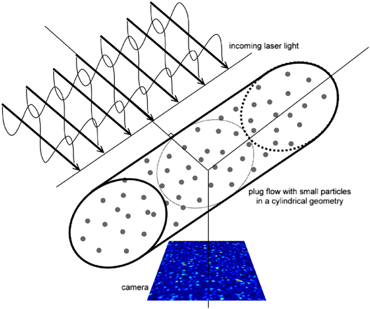
To study how K ≡ σI/〈I〉 depends on V, we use a simple cylindrical geometry with plug flow (i.e., a uniform constant velocity profile). The cylinder is 1 cm long with a 1 mm radius, which is characteristic for the external carotid artery.
![]()
Figure 1.Simulation setup: a plane wave is incident on a cylindrical geometry filled with tiny spherical particles in motion. A “camera”, placed at a right angle, measures the resulting dynamic interferometric speckle pattern over time. Figure not to scale.
On the optics side of the code, we use a real refractive index of 1.52 for the spheres and 1.00 for the surrounding medium. The wavelength of illumination is 532 nm. The camera is placed at a distance of 25 cm from the cylinder, and is given a size of 1.25 cm by 5.00 cm with 1282 pixels.
2.2 Results
A study of the effect of velocity V and camera integration time T on the speckle contrast K is shown in
![]()
Figure 2.Speckle contrast K dependence on scatterer velocity V for various camera integration times T. The error bars show the spread (standard deviation) caused by 10 different sets of random initial particle positions.
As either V or T is increased, K decreases because more motion is captured. Generally speaking, the error is also lower for higher V and T, presumably because for those situations averaging occurs over a larger range of particle positions, which renders the random particle instantiations less relevant.
We hypothesize that the relevant parameter should in fact be d = VT, which is the physical distance the particles have travelled during the camera integration time.
![]()
Figure 3.Speckle contrast K dependence on scatterer “distance travelled”, d = VT. The data points are from
3 Theoretical comparison
Several analytical expressions for K are already well-known [
3.1 Theory
3.1.1 Speckle contrast dependence on decorrelation time
The analytical expressions are derived from the temporal fluctuation statistics of the speckles caused by the motion of the scatterers. Using the autocovariance of the temporal fluctuations
However, the difficulty in deriving an analytical expression is that the motion of the scatterers is usually a priori unknown or too complicated; therefore,
When a Lorentzian covariance is assumed, the speckle contrast is:
The Lorentzian equation is valid for unordered (Brownian) motion, whereas the Gaussian equation is more appropriate for ordered motion. Since those two types of motion are statistically independent, reality is likely somewhere between these two limits [
However, it is not yet clear whether these relationships are truly applicable in practice. An arguably more appropriate relationship for blood flow was derived while assuming a constant velocity [
3.1.2 Scaling of the decorrelation time with velocity
These expressions all give K as a function of τc, whereas the goal is to measure V. To that end, an expression for τc(V) is needed. It was postulated that τc scales inversely with V: [
3.2 Results
We may compare our results with these expressions by first noting that all expressions for K in equations
3.2.1 Speckle contrast dependence on decorrelation time
Having written K(τc/T) as K(w/d), equations
![]()
Figure 4.Speckle contrast versus (τc/T)/w = d−1. The data points are the same as in
From the figure, we note that the Lorentzian model describes our results poorly, whereas the other models do an excellent job for large τc/T ~ d−1 (low V). This is consistent with the fact that we have flow at a constant velocity, whereas the Lorentzian model is more appropriate for Brownian motion [
However, β describes the reduction of K due to the finite pixel size, whereas we have infinitesimal pixels. Therefore, we may not use β as a fitting parameter, and actually should just take β = 1, as is shown in
![]()
Figure 5.Speckle contrast versus (τc/T)/w = d−1. The data points are the same as in
Next, it may be seen that the Gaussian model performs slightly better across the whole domain than the constant-velocity model, although our simulations do have a constant velocity. A possible explanation could have been that particles move in and out of the laser’s view, which results in a small amount of speckle boiling. However, simulations without cyclic boundary conditions (in which we have a purely translational speckle) have revealed a less than 1% difference in the results; thus speckle boiling is not the cause.
Related to that, all models describe the results at small τc/T ~ d−1 (high V) poorly, as K seems to saturate in the simulations, which is why the fits were made for large d−1. However, fitting the models at small d−1 instead does not yield a good fit (not shown); therefore, the models cannot describe the simulations in this regime. In an experiment, the effect of static scatterers would be to increase the minimum contrast value [
3.2.2 Scaling of the decorrelation time with velocity
Finally, it is of prime interest to study the obtained value for the fitted w, as there exists disagreement in the literature. The hypothesised expressions for w in and just above of equation
| Used in | Used in | ||
|---|---|---|---|
| Model | w (m) | β (−) | w (β = 1) (m) |
| Lorentzian | – | – | 17.5 ± 0.2 |
| Gaussian | 12.6 ± 0.2 | 0.970 ± 0.004 | 11.8 ± 0.1 |
| const. vel. | 23.8 ± 0.3 | 0.955 ± 0.004 | 21.8 ± 0.2 |
Table 1. Used fit parameters of models
4 Conclusions
In summary, we have presented results of our new computer code, which simulates how a plane wave of coherent light scatters off of a collection of moving particles using Mie theory to form a dynamic interferometric speckle pattern (i.e., Laser Speckle Imaging (LSI)). By mimicking the finite integration time T of a real camera, we have shown how the speckle contrast K depends on particle velocity V and on T. Existing theoretical models already describe how K depends on the speckle decorrelation time τc and on T, and it is believed that τc = w/V; although the value of w is still disagreed upon in the literature. We provide evidence that τc does indeed scale inversely with V, and that wspeckle = λz/D (multiplied by an O(1) constant) is a very likely candidate for w. The Gaussian correlation model does an excellent job at describing our simulation results for large τc/T (low V), but deviates considerably for low τc/T (high V), for which we provide several hypotheses for future research. However, the Lorentzian model is unsuitable for ordered flow (i.e., advection). Other optical scattering techniques using photon correlation methodologies also have the continuing discussion about decomposing flow into advection and Brownian motion [
The strength of simulations, once validated, is that circumstances that are difficult to reach experimentally may be studied using numerical experiments. Therefore, in future research our computer code may be used to study the effect of all relevant parameters – and in particular those that are not easily accessible in experiments – which will help develop LSI as a fully quantitative non-invasive measurement technique for flowmetry in turbid media (e.g., blood flow
References
[1] J.D. Briers, S. Webster. Laser speckle contrast analysis (LASCA): a nonscanning, full-field technique for monitoring capillary blood flow. J. Biomed. Opt., 1, 174-180(1996).
[2] D.A. Boas, A.K. Dunn. Laser speckle contrast imaging in biomedical optics. J. Biomed. Opt., 15, 011109(2010).
[3] A.K. Dunn. Laser speckle contrast imaging of cerebral blood flow. Ann. Biomed. Eng., 40, 367-377(2012).
[4] M. Stern. In vivo evaluation of microcirculation by coherent light scattering. Nature, 254, 56(1975).
[5] M. Draijer, E. Hondebrink, T. van Leeuwen, W. Steenbergen. Review of laser speckle contrast techniques for visualizing tissue perfusion. Lasers Med. Sci., 24, 639(2009).
[6] K. Basak, M. Manjunatha, P.K. Dutta. Review of laser speckle-based analysis in medical imaging. Med. Biol. Eng. Comput., 50, 547-558(2012).
[7] T. Yoshimura. Statistical properties of dynamic speckles. J. Opt. Soc. Am. A, 3, 1032-1054(1986).
[8] T. Asakura, N. Takai. Dynamic laser speckles and their application to velocity measurements of the diffuse object. Appl. Phys., 25, 179-194(1981).
[9] A.F. Fercher, J.D. Briers. Flow visualization by means of single-exposure speckle photography. Opt. Commun., 37, 326-330(1981).
[10] Y. Wang, W. Lv, X. Chen, J. Lu, P. Li. Improving the sensitivity of velocity measurements in laser speckle contrast imaging using a noise correction method. Opt. Lett., 42, 4655-4658(2017).
[11] J. Rosen, D. Abookasis. Noninvasive optical imaging by speckle ensemble. Opt. Lett., 29, 253-255(2004).
[12] Y. Shinohara, T. Kashima, H. Akiyama, Y. Shimoda, D. Li, S. Kishi. Evaluation of fundus blood flow in normal individuals and patients with internal carotid artery obstruction using laser speckle flowgraphy. PloS One, 12, 0169596(2017).
[13] V. Lambrecht, M. Cutolo, F. De Keyser, S. Decuman, B. Ruaro, A. Sulli, E. Deschepper, V. Smith. Reliability of the quantitative assessment of peripheral blood perfusion by laser speckle contrast analysis in a systemic sclerosis cohort. Ann. Rheum. Dis., 75, 1263-1264(2016).
[14] V. Tuchin. Tissue optics: light scattering methods and instruments for medical diagnosis(2007).
[15] M.M. Qureshi, Y. Liu, K.D. Mac, M. Kim, A.M. Safi, E. Chung. Quantitative blood flow estimation in vivo by optical speckle image velocimetry. Optica, 8, 1092-1101(2021).
[16] A. Nadort, K. Kalkman, T.G. Van Leeuwen, D.J. Faber. Quantitative blood flow velocity imaging using laser speckle flowmetry. Sci. Rep., 6, 1-10(2016).
[17] D.D. Duncan, S.J. Kirkpatrick. Can laser speckle flowmetry be made a quantitative tool?. J. Opt. Soc. Am. A. Opt. Image. Sci. Vis., 25, 2088-2094(2008).
[18] R. Bandyopadhyay, A. Gittings, S. Suh, P. Dixon, D.J. Durian. Speckle-visibility spectroscopy: A tool to study time-varying dynamics. Rev. Sci. Instrum., 76, 093110(2005).
[19] D.D. Duncan, S.J. Kirkpatrick, J.C. Gladish. What is the proper statistical model for laser speckle flowmetry?. Complex Dynamics and Fluctuations in Biomedical Photonics V, 6855, 685502(2008).
[20] D. Briers, D.D. Duncan, E.R. Hirst, S.J. Kirkpatrick, M. Larsson, W. Steenbergen, T. Stromberg, O.B. Thompson. Laser speckle contrast imaging: theoretical and practical limitations. J. Biomed. Opt., 18, 066018(2013).
[21] O.B. Thompson, M.K. Andrews. Tissue perfusion measurements: multiple-exposure laser speckle analysis generates laser doppler-like spectra. J. Biomed. Opt., 15, 027015(2010).
[22] A.B. Parthasarathy, W.J. Tom, A. Gopal, X. Zhang, A.K. Dunn. Robust flow measurement with multi-exposure speckle imaging. Opt. Express, 16, 1975-1989(2008).
[23] J. Wang, Y. Wang, B. Li, D. Feng, J. Lu, Q. Luo, P. Li. Dual-wavelength laser speckle imaging to simultaneously access blood flow, blood volume, and oxygenation using a color CCD camera. Opt. Lett., 38, 3690-3692(2013).
[24] K. van As, J. Boterman, C.R. Kleijn, S. Kenjeres, N. Bhattacharya. Laser speckle imaging of flowing blood: A numerical study. Phys. Rev. E, 100, 033317(2019).
[25] M. Nemati, S. Kenjeres, H.P. Urbach, N. Bhattacharya. Fractality of pulsatile flow in speckle images. J. Appl. Phys., 119, 174902(2016).
[26] S.J. Kirkpatrick, D.D. Duncan, E.M. Wells-Gray. Detrimental effects of speckle-pixel size matching in laser speckle contrast imaging. Opt. Lett., 33, 2886-2888(2008).
[27] J.W. Goodman. Statistical properties of laser speckle patterns. Laser Speckle and Related Phenomena, 9-75(1975).
[28] J.W. Goodman. Statistical optics(2015).
[29] J. Briers, A. Fercher. Laser speckle technique for the visualization of retinal blood flow. Max Born Centenary Conf., 369, 22-29(1983).
[30] C. Wang, Z. Cao, X. Jin, W. Lin, Y. Zheng, B. Zeng, M. Xu. Robust quantitative single-exposure laser speckle imaging with true flow speckle contrast in the temporal and spatial domains. Biomed. Opt. Express, 10, 4097-4114(2019).
[31] V.N.D. Le, V.J. Srinivasan. Beyond diffuse correlations: deciphering random flow in time-of-flight resolved light dynamics. Opt. Express, 28, 11191-11214(2020).


Set citation alerts for the article
Please enter your email address

© Copyright 2018-2021 | Chinese Laser Press. All Rights Reserved 沪ICP备15018463号-20