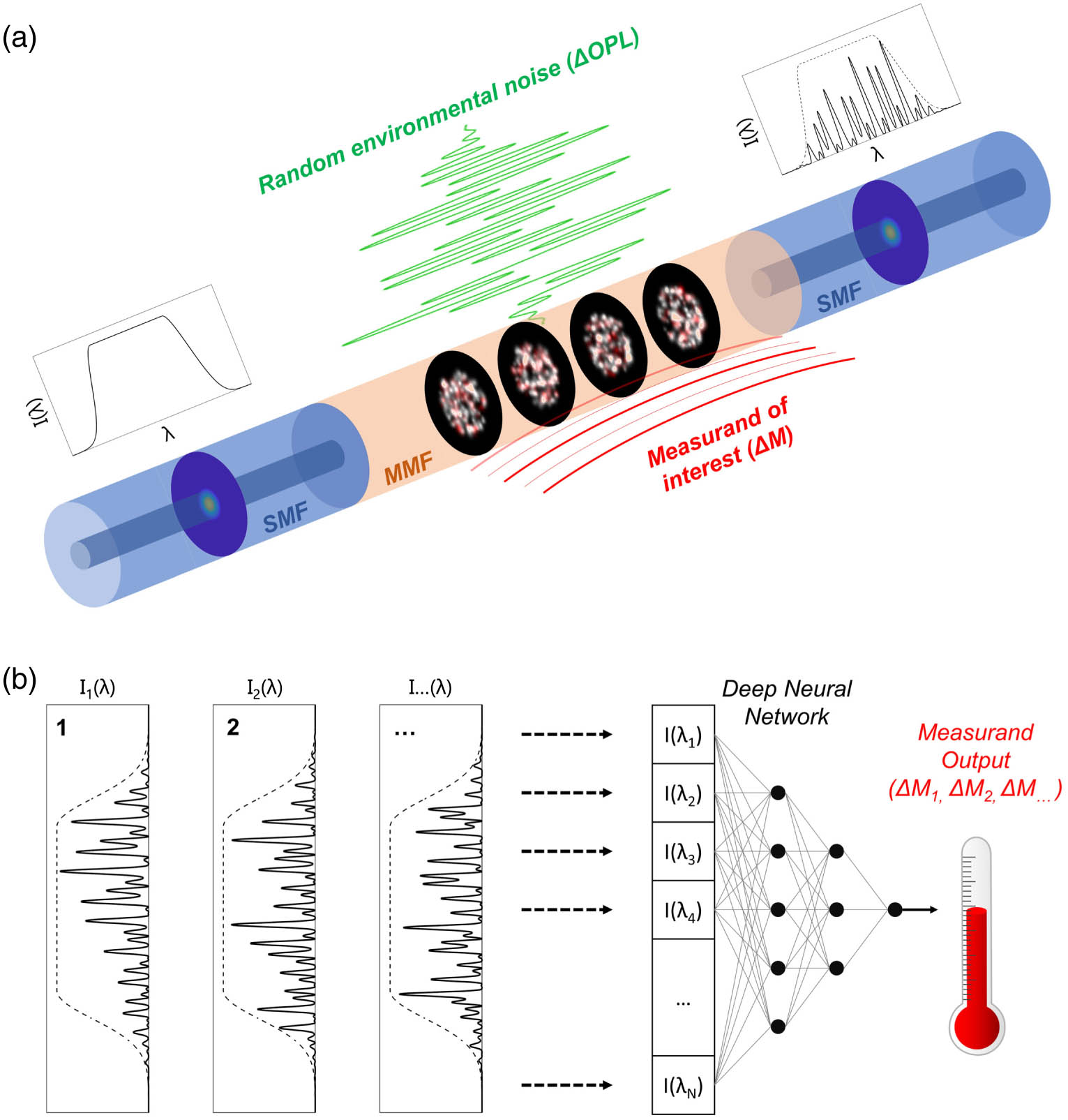
Fig. 1. Schematic diagram of specific measurement under strong noise using MMF and DNN. (a) An SMF-MMF-SMF structure is used to realise complex interference spectra from MMF with a broadband input. The sensing MMF is subjected to both changes in the measurand and strong noise to create complex changes in the output interference spectrum. The speckle images in the MMF conceptually show the impact of the measurand (red), which may be relatively small compared to the noise (white). (b) Various spectra together with their corresponding measurand labels are used to train a DNN. Once trained, the DNN is able to predict the measurand value buried within each interference spectrum.

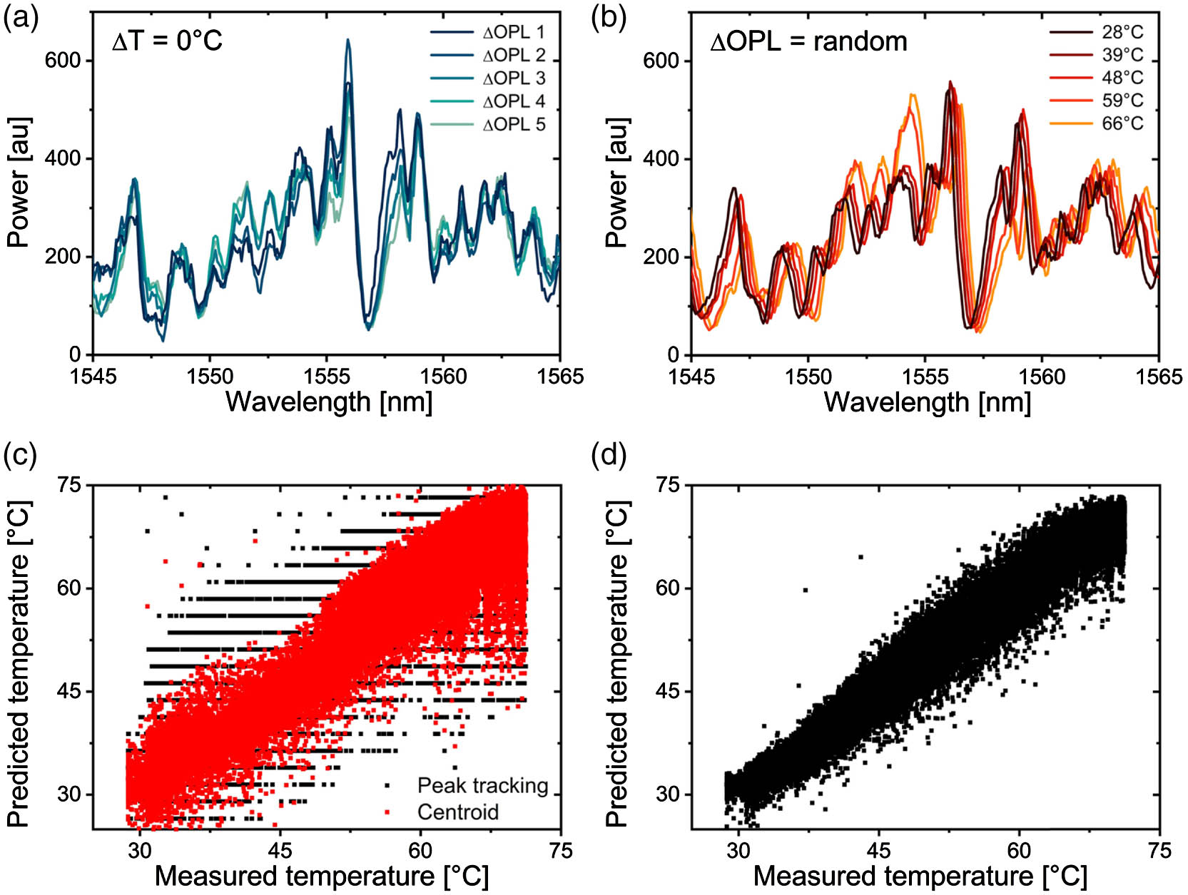
Fig. 2. Complex cross-sensitivity problem in specific measurement with MMF-based sensors under OPL noise. (a) Transmission interference spectra from the SOF at a fixed temperature under white noise in OPL created by shaking the loosely mounted SOF. (b) Interference spectra at several temperatures under OPL noise. (c) Predicted (calibrated) temperature by peak tracking (black) and after applying a centroid function to improve the accuracy (red). (d) Predicted (calibrated) temperature obtained using a Fourier phase-shift technique. The measured temperature in (c) and (d) was obtained using a reference thermocouple.

Fig. 3. Schematic diagram of the multilayer perceptron (MLP) architecture used in this work. After being trained using thousands of different noisy MMF interference spectra with their corresponding temperature labels, the trained model takes an MMF spectrum as its input and produces a predicted temperature value at its output.

Fig. 4. Comparison of temperatures predicted from the trained MLP using SOF interference spectra as input and measured temperatures under OPL noise. (a) Training and testing on the same temperature range using the short temperature range from 30°C to 70°C (T1) with 8400 testing examples (data points). (b) Training and testing on the same temperature range using extended temperature range from 30°C to 630°C (T2) with 7845 testing examples. (c) Same procedure but training and testing on different data sets, the MLP is trained on the short temperature range and tested on the extended temperature range, where many temperature values are out of the training range. (d) The MLP is trained on the extended temperature range and tested on the short temperature range. In this case all the testing temperatures are predicted within the range of the training set but with less accuracy compared with (b) due to a shift in the data set.

Fig. 5. Mitigating the domain shift issue using a combined data set T1 + T2. (a) The testing set was T1 using 8400 example spectra. (b) The testing set was T2 using 7845 example spectra. The test results were improved for both cases.

Fig. 6. Comparison between MLP and CNN architectures with a similar number of parameters. Training and testing were done in the same manner as in Figs. 4 and 5. The CNN produces inferior predictions compared with its MLP counterpart, indicating that the raw interference spectra from the highly multimode SOF do not possess significant wavelength locality.

Fig. 7. Experimental setup. The SOF was mounted loosely inside the SS tube so that it vibrated within the SS tube. The shaker was driven by a white noise vibration profile. The SS tube was placed centrally within a tube furnace and the temperature referenced with a thermocouple.

Fig. 8. Schematic diagram of the 1D CNN architecture.

Table 1. Temperature Measurement Accuracy for Different Calibration Methods^a

Table 2. Data Set Used for Training and Testing