Shaochong Wu, Hongyuan Wang, Zhiqiang Yan. Optical system design method of the all-day starlight refraction navigation system[J]. Journal of the European Optical Society-Rapid Publications, 2023, 19(2): 2023041
Copy Citation Text
The application of starlight refraction navigation to spacecraft and space weapons is a significant development direction. Observing enough refracted stars for the star sensor in a strong limb background is an urgent problem. The all-day optical system parameters are analyzed based on the star detection requirement and navigation accuracy. Combined with primary aberration theory, the prime-focus catadioptric optical system is selected to meet the design requirements of a wide field of view (FOV) and tight structure. An H-band (1.52 μm–1.78 μm) star sensor is designed with an FOV of 6°, a focal length of 831 mm, an effective aperture of 253 mm, and a relative distortion of 0.03%. The energy concentration of the star point is 85% within 30 μm, and the maximum lateral chromatic aberration is 2.9 μm, which meets the imaging requirements. Furthermore, a baffle is designed to avoid the influence of direct sunlight on stellar imaging. The proposed method can provide a theoretical foundation and technical support for the optical design of the refraction star navigation.
Under the condition of Global Navigation Satellite System (GNSS) rejection, starlight refraction navigation can still provide position and attitude information for satellites and space weapons [1]. More and more researchers have paid considerable attention to this promising autonomous celestial navigation [2, 3]. In the starlight refraction navigation system, the star sensor observes three non-refracted stars to solve the attitude. Combined with the refracted stars at tangent heights from 20 km to 50 km, the position information can be obtained further [4]. Star sensors can measure the height based on one refracted star. It can simultaneously calculate the height, longitude, and latitude based on three refracted stars. Starlight refraction navigation can also be used to suppress accumulated errors in inertial navigation systems and improve the accuracy of integrated navigation systems [5].
Scholars have conducted in-depth research on starlight refraction navigation algorithms, but they overlook the issue of how star sensors observe refracted stars in strong limb backgrounds during the day. In 2002, the ESA GOMOS satellite could observe 4th magnitude stars in a bright limb background [6], with an optical aperture of 300 mm and a focal length of 1.05 m. Because it uses the Cassegrain optical system, the field of view (FOV) is limited to 0.6°. The FOV is too small to detect enough refracted stars. Based on the principle of autonomous navigation, Wu et al. [7] designed a star sensor working in the visible light band in 2015. Because the number of stars in the H-band is much greater than that in the visible band, Xu and Jiang [8] designed an infrared optical system with an FOV of 4°. In 2020, Jiang et al. [9] gave an optimization method for the optical system with a 5.8° FOV. This star sensor had a 57.5% probability of observing refracted stars at night. In 2020, Bai et al. [10] designed a visible catadioptric star sensor for the satellite with an aperture of 285 mm for lenses, an FOV of 2.8°, and an aperture of 257 mm for mirrors. Because the strong limb background during the day is ignored, the existing star sensors [7–10] were unable to detect enough refracted stars during the day.
The design method of all-day star sensors for starlight refraction navigation has not been proposed, but researchers have studied many all-day star sensors that work near the ground. In 1964, the United States designed a star sensor [11] with an aperture of 400 mm. It can measure 7th magnitude stars at night and 3rd magnitude stars during the day. In 2002, the Blast star sensor [12] was designed with an aperture of 100 mm and a baffle of 1.2 m, and the baffle is used to suppress the solar stray light. Compared to the visible band, the sky background radiance in the infrared band is weaker [13], and scholars often use infrared star sensors to suppress the bright background. The ST star sensor [14] worked in the near-infrared light band, with an aperture of 180 mm, a focal length of 1800 mm, and an FOV of 19.5′. In 2005, Microcosm Company [15] designed a near-infrared star sensor, which can observe 7th magnitude stars. In 2021, Wang Bingwen et al. proposed an optical system design method for star sensors in the H-band (1.52 μm–1.78 μm) with the catadioptric optical system, an aperture of 200 mm, an FOV of 0.8°, an integration time of 0.35 s, and a focal length of 1174 mm [16]. The baffle is needed to suppress the solar stray light, and the baffle’s length is often more than three times the aperture. And the larger the FOV, the longer the baffle [17]. The existing all-day star sensor cannot meet the requirements of starlight refraction navigation due to the small FOV or long integration time.
In general, all-day star sensors have the characteristics of long focal lengths and large apertures. The H-band and the catadioptric system are more suitable for designing all-day star sensors. And the all-day star sensors for starlight refraction navigation have not been studied. This paper proposes an optical system design method for the all-day starlight refraction navigation system to meet the autonomous navigation. The article is arranged as follows. Section 2 introduces the principle of starlight refraction navigation. Section 3 proposes the method for determining the parameters of star sensors, including the FOV, limit magnitude, aperture, focal length, and optical system structure. Section 4 introduces the design results of the star sensor. The star sensor works in the H-band and adopts the prime-focus catadioptric optical system. The designed optical system is tighter than the refractive system. It contains fewer lenses, and only the spherical lenses are used to correct aberrations. Section 5 provides a summary of this paper.
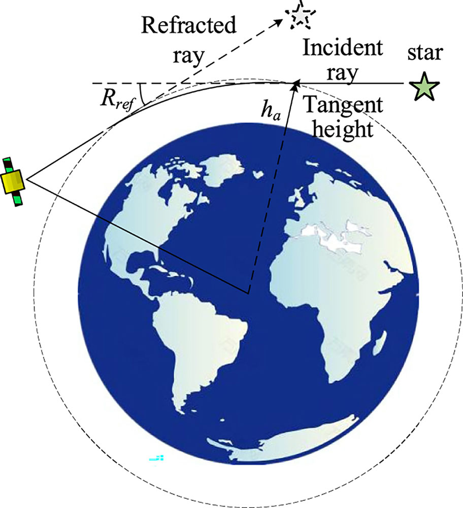
2 Principle of starlight navigation
As shown in Figure 1, due to the uneven density of the atmosphere, the starlight passing through the Earth’s atmosphere will bend to the Earth. The angle Rref between the incident and refracted ray is the starlight refraction angle. The navigation algorithms use starlight refraction angles to sense the earth’s horizon and get the satellite’s position based on at least three stars.
Figure 1.The principle of starlight refraction for navigation.
The star refraction angle can be obtained as follows [18]:where Rref is the starlight refraction angle, ha is the tangent height between 20 km and 50 km. The tangent height is nearest height of the ray path from the earth.
The position information can be obtained with the refracted stars at tangent heights from 20 km to 50 km. For the height above 50 km, the refraction angle is too small to be measured. For heights below 20 km, the changes in atmospheric density are pretty drastic, and the refraction angle is unsuitable for navigation [18]. The accuracy of star sensors directly determines the navigation accuracy. The refraction angle at the tangent height of 20 km is 316.31″, and the measurement error of 4.74″ will cause a navigation error of 64 m [19]. The star sensor needs to observe non-refracted stars for high-precision attitude measurement and detect the refracted stars near the Earth for the position. Therefore, the FOV, limit magnitude, and image quality of the star sensor for starlight refraction navigation are pretty different from those of traditional star sensors.
3 Main parameter design method
In order to meet all-day autonomous navigation, the star detection requirement is analyzed, as shown in Figure 2. The relationship of FOV and limit magnitude is determined to satisfy the detection requirement. Then the aperture and focal length is analyzed to meet the limit magnitude. Combined with the image quality requirement, the appropriate system structural parameters are selected. Finally, the initial parameters of the optical system are determined and given to meet the starlight refraction navigation.
Figure 2.Diagram of the main parameter design method.
For the star sensor, the FOV is divided into two parts, namely the non-refracted region and refracted region, which meet the needs of attitude calculation and position calculation respectively, as shown in Figure 3. In Figure 3a, the subscript t represents the northeast coordinate system, and the solar zenith angle is 0° in this paper [20]. The tangent height of the refracted star ranges from 20 km to 50 km. When the satellite’s height is 400 km, the field of view w0 covering the atmospheric is very small. In order to optimize the FOV configuration, one of the edges of the detector is placed in the tangential direction of the earth, as shown in Figure 3b.
Figure 3.FOV distribution of the star sensor. (a) Geometry model of starlight refraction; (b) layout of FOV distribution.
The probability Pu of detecting stars to meet the requirements of starlight refraction navigation is as follows:where Nr is the number of refracted stars, and Nn is the number of non-refracted stars.
In this paper, the requirement of the star detection probability is Pu > 85%. As shown in Figure 3b, the non-refracted region is larger than the refracted region, and its limit magnitude is larger. So, it only needs to meet the requirement that the refracted star is more than three.
In order to fully utilize the FOV of the star sensor, this paper adopts a circular FOV star sensor. As shown in Figure 3, the area Sd of the refracted region is as follows:where ha = 20 km, hb = 50 km, α and β is the angle between the optical axis direction and the center of the earth earth [21], β is shown in the Figure 3a. Re is the earth radius. hs is the satellite height which is assumed to be 400 km.
3.1.2 Image quality requirement
The image quality requirements of star sensors mainly include distortion and energy distribution. Distortion determines the navigation accuracy of the system, and energy distribution mainly determines the detection ability of star sensors. The energy distribution is mainly related to spherical aberration, dispersion, and astigmatism.
Distortion
From the previous analysis, the refraction angle error of 4.74″ will cause a position error of 64 m at the tangent height of 20 km. In order to limit the navigation error to less than 100 m, the error caused by distortion should not exceed 4.74″ with an FOV of 6°. And the distortion δrel should not exceed 0.043% by the equation (4):where R20 km is the starlight refraction angle at the tangent height of 20 km.
Energy distribution
The star point on the image surface shouldn’t be a point, but a diffuse spot with a certain size for the star point extraction algorithm [22]. The shape of the star point should be approximately circular, and the energy is close to normal distribution. When the size of the diffuse spots is 3 × 3 pixels, the corresponding centroid positioning accuracy is 0.001 pixels which can meet the use. And it is required that the 85% energy of the diffusion spot is within the 3 × 3 pixels.
3.2 Optical system parameters
3.2.1 FOV and limit magnitude
The FOV and the limit magnitude determine the probability of star detection. Therefore, the FOV and limit magnitude are analyzed first. The limit magnitude is related to the background noise electrons Nb and star electrons Nsm observed by the star sensor. The number of electrons of the star is:where K is a coefficient representing the concentration ratio of light. When 85% of the star energy is concentrated in 3 × 3 pixels, K is 1/9. D denotes the effective aperture of the optical system; h denotes the Planck constant; c denotes the speed of light; τopt denotes the transmittance of the optical system; t is the integration time; Em (λ) is the spectral irradiance of the star magnitude m. λ is the wavelength; λ1 is lower limit of wavelength integration; λ2 is upper limit of wavelength integration; Q(λ) is the quantum efficiency; τatm (λ, ht) is the transmittance of atmospheric at different tangential heights ht.
The magnitude relationship is:where E0 is the spectral irradiance of the zero magnitude [13].
The limb background radiation includes the solar reflection radiation, Earth radiation, Earth reflection radiation and the atmospheric radiation. The number of electrons for the limb background is:where u is the pixel size of the detector, and f is the focal length of the optical system. ψ(λ, ht) is the atmospheric limb background radiance data at the tangent height ht.
The signal-to-noise ratio (SNR) [16] is shown in equation (8). A signal-to-noise ratio of 5 or more is sufficient for star point extraction:where is the squared photoelectrons of detector noise, and Vth is the threshold.
The limb background radiation is not constant, but decreases with the increasing tangent height. The MODTRAN5 software [23] is used to calculate the limb radiance. Figure 4 shows the limb background radiance at different tangent heights at 1.65 μm.
Figure 4.Limb background radiance at different tangent heights at 1.65 μm.
Because the limb background radiance is variable, the corresponding limit magnitude varies with height. As shown in equation (9), the limit magnitude at the tangent height ha is ml_ha by solving equation (8). The limit magnitude at the tangent height hb is ml_hb shown in equation (10). So, the limit magnitude difference at different tangent heights can be calculated according to equation (11). Since the detector noise is much smaller than the limb background Nb, can be ignored in the calculation:where Nb_ha is the limb background at the tangent height of ha, and Nb_hb is the limb background at the tangent height of hb.
The simulation is used to analyze the limit magnitude with different FOV meeting the star detection requirement. The optical axis pointing of the star sensor is shown in Figure 3. The attitude and position of the star sensor are randomly changed in the simulation, and the corresponding limit magnitude of different FOV is calculated to meet the star detection requirement Pu > 85%, as shown in Table 1. In the simulation, the navigation stars are selected from the H-band catalog, and the tangent height is 20–50 km. It can be seen that the limit magnitude decreases with the increasing FOV. Table 1 shows the limit magnitude at 20 km, and the limit magnitude at other tangent heights is calculated by the equation (11).
Table Infomation Is Not Enable
Assuming that the navigation stars are uniformly distributed, the number NFOV of refracted stars [24] in the refracted region can be calculated by equation (12):where N(mlim) is the number of stars corresponding to the limit magnitude mlim.
The probability Pn of at least n refracted stars appearing in the refracted region [25] can be calculated by equation (13). The number of stars in the H-band is much greater than that in the visible band [16]. Therefore, H-band star sensors are better than the visible band to meet the needs of refracted star detection according to equations (12) and (13):
Because the limb background varies at different heights, the limit magnitude at 30 km is used to predict the probability of star detection by the equations (12) and (13). Figure 5 shows the detection probabilities of refracted stars corresponding to different limit magnitudes at 20 km with a 6° FOV. It can be seen that the simulation results and prediction results by equation (13) are basically consistent.
Figure 5.Star detection probability at different limit magnitude with 6° FOV.
According to the equations (5)–(8), the limit magnitude is determined by the aperture, focal length, and some detector parameters. Most infrared detectors have similar parameters, with pixel sizes ranging from 7 μm to 15 μm. This paper discusses the aperture and focal length based on a 10 μm pixel size.
Substituting the equations (5) and (7) into (8) to get:
Based on the detector [26] shown in Table 2 and the limit magnitude in Table 1, the aperture and focal length for different FOV are calculated through simulation by the trial, as shown in Figure 6 and Table 3. The transmittance of the optical system is assumed to be 85%. The equation (14) is used to predict the aperture and focal length. It can be seen that the simulation results and prediction results are basically consistent. The F-number is the ratio of the focal length to the aperture.
Figure 6.The aperture and focal length with different FOV meeting the star detection requirements.
Table Infomation Is Not EnableTable Infomation Is Not Enable
Table 3 can be used for the selection of optical system structures. The optical system of the star sensor usually adopts refractive, reflective, and catadioptric structures. The F-number of the refractive optical systems is often less than 2 with a large FOV. The aperture of the optical system needs to reach 200 mm even in a 15° FOV. In order to correct distortions and astigmatism in a large FOV, more than ten refractive lenses are often used in refractive optical systems. And the baffle corresponding to the large FOV is also cumbersome. The F-number of reflective optical system is often greater than 3, with the advantage of large aperture and long focal length, but their FOV is often small. The catadioptric optical system can expand the FOV of the reflective optical system with corrector lenses, so this paper initially selects the catadioptric optical with a medium FOV of 6°, and the F-number is 3.
3.2.3 Optical system structure
This paper intends to design an optical system based on a catadioptric optical system. The basic structure of the two-mirror optical system is shown in Figure 7. h1 is the half aperture of the prime mirror. h2 is the half aperture of the second mirror. l2 is the distance from the second mirror to the prime focus. l′2 is the distance from the second mirror to the second focus. f′1 is the primary mirror’s focus length.
Figure 7.Basic structure of two-mirror optical system.
Both the primary mirror and the secondary mirror are the type of conic:where e2 is the eccentricity of the curve, r is the curvature radius at the curve vertex.
Define two parameters α and β related to overall dimensions:
From aberration analysis, the spherical aberration, astigmatism, and distortion seriously restrict the FOV of the optical system [27]. According to the third-order aberration coefficients of Seidel [16], it should meet the following equation:where S1 is the coefficient of the spherical aberration, S3 is the coefficient of the astigmatism, and S5 is the coefficient of the distortion. e1 is the curve eccentricity of the prime mirror, e2 is the curve eccentricity of the second mirror.
Based on equations (16) and (17), it can be obtained:
The only valid solution of equation (18) can be obtained as follows:
Equation (19) indicates that the prime-focus optical structure with one mirror can eliminate the astigmatism and distortion, so as to expand the FOV of the catadioptric system. The prime-focus optical system has been well applied in the large aperture telescope [28] with a 4 m aperture.
Based on the analysis method in this section, the following optical system parameters have been preliminarily determined, as shown in Table 4.
Table Infomation Is Not Enable
4 Optical system design and result
According to the initial parameters of the optical system, the optical system is designed and optimized. The image quality and stray light suppression performance are evaluated.
4.1 Optical system design result
Wide-field corrector is added to the prime-focus optical system to further correct aberrations and expand the FOV. The optical design result is Terebizh-style [29] with five spherical lenses, as shown in Figure 8 and Table 5.
Based on the optimization method in Zemax, the surface shape parameter e2, curvature radius, and interval of the lenses are taken as optimization variables, and RMS + Wavefront + Centroid are used as the optimization function. The optical system operates in a vacuum environment. Operand effective focal length (EFFL) controls the range of focal length. Operand axial color (AXCL) controls the lateral chromatic aberration. Operand RMS spot radius with respect to the geometric image centroid (RSCE) controls the size of the spot diagram. Operand DIMX is used to control the distortion. Operands COMA and ASTI are used to control coma aberration and astigmatism. During the design, the parameter range is limited by the above operands. Through repeated optimization, the optical system result was ultimately obtained. The surface shape parameter of the mirror is −2.674. The glasses are from the CDGM glass warehouse. The focal length of the designed optical lens is 831 mm, the aperture is 300 mm, and the transmittance is 59%. Due to the obstruction of the lens, the effective aperture is 253 mm, whose corresponding transmittance is 85.3% in the equation (14). The length of the optical system is 1038 mm, the aperture is 300 mm, and the weight is 3.1 kg.
4.2 Image quality
The spot diagram, encircled energy curves, chromatic aberration curves, and distortion curves are used to evaluate the imaging quality of the optical system for the star sensor.
In the spectral range of 1.52–1.78 μm, Figure 9 shows the spot diagrams of the diffuse spots under five FOVs of 0.0°, 0.8°, 1.5°, 2.2° and 3.0°. Table 6 shows the RMS radius and GEO radius of the diffuse spots. It is clearly seen that the distributions of the diffuse spots were not only basically round and concentrated, but also had a certain degree of dispersion and good symmetry. The RMS radius of the diffuse spots is smaller than the pixel size.
The curves of the encircled energy under the different FOVs are shown in Figure 10. The energy distributions of the diffuse spots are close to the Gaussian normal distribution. Eighty five percent of the energy contained in the diffuse spots is distributed within a radius of 13.3 μm, which is less than the 3 × 3 pixels and meets the design requirement. Ninety percent of the energy is distributed within the 3 × 3 pixels. Figure 11 shows the lateral chromatic aberration between different wavelengths (1.52–1.78 μm) and the center wavelength of 1.65 μm. The results show that the maximum lateral chromatic aberration was 2.9 μm, which is less than the airy radius of 5.4 μm, and can meet the requirements.
Figure 10.Energy concentration curve of the designed optical system.
For the optical system of the star sensor, the smaller relative distortion is necessary to obtain a higher measurement accuracy. The relative distortion curve of the optical system is shown in Figure 12. The maximum relative distortion is 0.025% in the FOV from −3° to +3°, which fully meet the design specification of the relative distortion 0.043%.
Figure 12.Relative distortion curves of the designed optical system.
Tolerance analysis is one of the most important steps in optical design. Table 7 shows the tolerances for the designed optical system, which is obtained from a large catadioptric optical system [10, 30]. Tolerance analysis is performed by the ZEMAX software with two methods, including sensitivity analysis and Monte Carlo analysis. The adjustment parameter (compensator) and the performance criteria are the back focus and RMS spot. Table 8 shows the results of tolerancing by sensitivity analysis method. It shows that 90% of tolerances have an RMS spot radius of 8.25 μm. Furthermore, 80% of tolerances lead to an RMS spot radius of 7.83 μm, which is satisfying with a 10 μm pixel pitch.
Table Infomation Is Not EnableTable Infomation Is Not Enable
4.3 Stray light suppression
In order to reduce the adverse impact of stray light sources, mainly from the sun, a baffle is designed by the method in [17], as shown in Figure 13. The surface of the baffle is sprayed with Metal Velvet, which has an absorption rate better than 96% at the H-band. The stray light analysis software Lightools is used to evaluate the performance of the stray light elimination system with PST [16] as the evaluation index. PST is the ratio of light received by the optical system to sunlight. The off-axis angle is the angle between the sun and the optical axis. Set the off-axis angle of 5°–80° and a step size of 5°. The obtained PST curve with the off-axis angle is shown in Figure 14. With the increase of off-axis angle, the PST decreases. When the off-axis angle is greater than 30°, the PST is better than 10−6, and the influence of direct solar light on star detection will be negligible [16].
It can be seen that the baffle also acts as a tube, and the designed system is tighter than the refractive system. It contains fewer lenses, and only the spherical lenses are used to correct aberrations.
5 Conclusion
In order to meet all-day autonomous navigation, an optical system design method of the starlight refraction navigation system is proposed in this paper. Based on the optical system requirement, the method for determining the optical system parameters and structure is presented. An H-band catadioptric star sensor is designed. Compared with the refractive optical system, the designed catadioptric system uses fewer lenses, and the structure is tighter. The proposed method can provide a theoretical foundation and technical support for the optical design of the refraction star navigation. Next, we will build a hardware-in-the-loop simulation platform and verify relevant navigation algorithms.
References
[1] X. Ning, X. Sun, W. Chao. Integration of star pixel coordinates and their time differential measurement in satellite stellar refraction navigation. Acta Astronaut., 159, 286-293(2019).
[2] H. Wang, S. Wu, B. Wang, Z. Yan, S. Yao, C. Zeliu. Near-infrared star map simulation for starlight refraction sensor based on ray tracing. Infrared Phys. Technol., 132, 104760(2023).
[3] S. Wu, H. Wang, B. Wang. Construction of a backpropagation starlight atmospheric refraction model based on ray tracing. Appl. Opt., 62, 3778-3787(2023).
[4] J. Anthony. Air Force Phillips Laboratory autonomous space navigation experiment. AIAA, Space Programs and Technologies Conference, Huntsville, AL, March 24–27, 1992, 9(1992).
[5] D. Wang, H. Lv, X. An, W. Jie. A high-accuracy constrained SINS/CNS tight integrated navigation for high-orbit automated transfer vehicles. Acta Astronaut., 151, 614-625(2018).
[6] J.L. Bertaux, E. Kyrölä, D. Fussen, A. Hauchecorne, F. Dalaudier, V. Sofieva, R. Fraisse. Global ozone monitoring by occultation of stars: an overview of GOMOS measurements on ENVISAT. Atmos. Chem. Phys., 10, 12091-12148(2010).
[7] Y. Wu, X. Zhang, J. Zhang, L. Wang, F. Zeng. Research on the autonomous star sensor based on indirectly sensing horizon and its optical design. Acta Optica Sinica, 35, 266-275(2015).
[8] L. Xu, J. Jiang. The analysis for the influence of the refracted star detection. Presented at 2018 IEEE CSAA Guidance, Navigation and Control Conference (CGNCC), 1-8(2018).
[9] J. Jiang, Y. Ma, G. Zhang. Parameter optimization of a single-FOV-double-region celestial navigation system. Opt. Express, 28, 25149-25166(2020).
[10] Y. Bai, J. Li, R. Zha, Y. Wang, G. Lei. Catadioptric optical system design of 15-magnitude star sensor with large entrance pupil diameter. Sensors, 20, 5501(2020).
[11] M. Dachs, A. Parr. Day/night shipborne test range star tracker (Shipborne day/night star tracker assisting Missile Guidance System monitoring in Atlantic and Pacific Missile Ranges), 346-373(1970).
[12] R.W.H. van Bezooijen. SIRTF autonomous star tracker. IR Space telescopes and instruments, 4850(2003).
[13] Z. Liao, Z. Dong, H. Wang, X. Mao, B. Wang, S. Wu, Y. Zang, Y. Lu. Analysis of flow field aero-optical effects on the imaging by near-earth space all-time short-wave infrared star sensors. IEEE Sens. J., 22, 15044-15053(2022).
[14] S. Poppi, C. Pernechele, M. Morsiani, J. Roda, V. Chiomento, E. Giro, A. Frigo, T. Pisanu, S. Righini, L. Traverso. An optical telescope to achieve a tracking and pointing model for radiotelescopes(2007).
[15] C.A. Nardell, J. Wertz, P.B. Hays. Image processing, simulation and performance predictions for the MicroMak star tracker. Proc SPIE, 5916, 59160U-59160U-12(2005).
[16] B. Wang, H. Wang, X. Mao, S. Wu, Z. Liao, Y. Zang. Optical system design method of near-Earth short-wave infrared star sensor. IEEE Sens. J., 22, 22169-22178(2022).
[17] M. Asadnezhad, A. Eslamimajd, H. Hajghassem. Optical system design of star sensor and stray light analysis. J. Eur. Opt. Soc. – Rapid Publ., 14, 1-11(2018).
[18] X. Wang, J. Xie, S. Ma. Starlight atmospheric refraction model for a continuous range of height. J. Guid. Control. Dynam., 33, 634-637(2010).
[19] R.L. White, S.W. Thurman, F.A. Barnes. Autonomous satellite navigation using observations of starlight atmospheric refraction. J. Navig., 32, 317-333(1985).
[20] H. Wang, S. Wu, Z. Ye, X. Zheng, S. Sun, B. Wang, Y. Zang, X. Zhang. Research on joint calibration and compensation of the inclinometer installation and instrument errors in the celestial positioning system. J. Field Robot., 39, 1151-1161(2022).
[21] H.M. Qian, L. Sun, J.N. Cai, W. Huang. A starlight refraction scheme with single star sensor used in autonomous satellite navigation system. Acta Astronaut., 96, 45-52(2014).
[22] J. Jiang, H. Wang, G. Zhang. High-accuracy synchronous extraction algorithm of star and celestial body features for optical navigation sensor. IEEE Sens. J., 18, 713-723(2017).
[23] A. Berk, G.P. Anderson, P.K. Acharya, L.S. Bernstein, L. Muratov, J. Lee, M. Fox, S. Adler, J. Chetwynd, M. Hoke, R. Lockwood, J. Gardner, T. Cooley, C. Borel, P.E. Lewis. MODTRAN5: a reformulated atmospheric band model with auxiliary species and practical multiple scattering options: update. Proc. SPIE, 5806, 662-667(2005).
[24] C.C. Liebe. Accuracy performance of star trackers-a tutorial. IEEE Trans. Aerospace Electron. Syst., 38, 587-599(2002).
[25] W.U. Yanxiong, W.A.N.G. Liping. Optical system of star sensor with miniaturization and wide spectral band. J. Appl. Opt., 42, 782-789(2021).
[26] A. Menduiña Fernández. Measuring and calibrating non-common path aberrations in adaptive optics assisted image-slicer based spectrographs. Doctoral dissertation(2021).
[27] F.E. Ross. Lens systems for correcting coma of mirrors. Astrophys. J., 81, 156(1935).
[28] S. Kent, R. Bernstein, T. Abbott, B. Bigelow, D. Brooks, P. Doel, B. Flaugher, M. Gladders, A. Walker, S. Worswick. Preliminary optical design for a 2.2 degree diameter prime focus corrector for the Blanco 4 meter telescope. Ground-based and Airborne Instrumentation for Astronomy. Proc. SPIE, 6269, 626-937(2006).
[29] V.Y. Terebizh. On the capabilities of survey telescopes of moderate size. Astron. J., 152, 121(2016).
[30] J. Li, G. Lei, Y. Bai. Optical path design for catadioptric star sensor with large aperture. Acta Photonica Sinica, 49, 0611002(2020).
Shaochong Wu, Hongyuan Wang, Zhiqiang Yan. Optical system design method of the all-day starlight refraction navigation system[J]. Journal of the European Optical Society-Rapid Publications, 2023, 19(2): 2023041