Quantum Fisher information of triphoton states

Tao Li; Mingyang Li; Junming Huang

doi:10.3788/COL201614.032701

Abstract

Based on the standard angular momentum theory, we create an experiment on preparing maximally path-entangled

{(| N, 0 + | 0, N)}^{2}

(NOON) states of triphotons. In order to explain the error between the theoretical and experimental data, we consider the background events during the experiment, and observe their effect on the uncertainty in

{\hat{S}}_{1}

. Afterwards, we calculate the quantum Fisher information (QFI) of the states to evaluate their potential applications in quantum metrology. Our results show that by adding the appropriate background terms, the theoretical data of the produced states matches well with the experimental data. In this case, the QFI of the states is lower than maximally entangled NOON states, but still higher than a classical state.

Polarization squeezing and the quantum entanglement of a light field have been concerns for decades because of their significance in fundamental physics and its potential applications in quantum metrology and quantum information^[1–6]. Formally, squeezing is defined as a reduction of the polarization uncertainty below the shot-noise limit, which is the standard quantum limit imposed by the Heisenberg uncertainty relationship. It is generally thought that squeezing, which is closely related to multipartite entanglement, arises from the quantum correlation effect among individual particles^[7–10]. Quantum metrology based upon maximally entangled ${(| N, 0 〉 + | 0, N 〉)}^{2}$ (NOON) states leads to super-resolving phase estimations^[11,12]. However, an ideal optical source of entangled states is still unattainable because of technical difficulties^[13]. By applying various state-projection measurements, a lot of groups have realized few-photon NOON states so far^[4,14–18]. In particular, Shalm et al. have succeed in preparing maximally entangled NOON states of triphotons^[18]. They looked into the uncertainty in the Stokes parameters, but we found that there is a certain degree of error between the theoretical curve and the experimental data, indicating that the obtained states are not pure NOON states. To explain the error, in this Letter, we theoretically study the producing process of the triphotons and add background terms into the states.

Since the obtained states are not pure NOON states, its capacity as an input state in phase estimations may decrease, which needs to be measured. A typical phase estimation includes three steps^[19]. First, the input state of the sensor, described by its density operator ${\hat{ρ}}_{in}$ , is prepared. Then, the sensor undergoes the phase-dependent dynamical process $\hat{U} (ϕ)$ and evolves to the output state ${\hat{ρ}}_{out}$ . Finally, a measurement is made of the output state, and the outcome $x$ is used by suitable data processing to produce an unbiased estimator $\hat{ϕ} (x)$ of the parameter $ϕ$ . The precision of the estimation is described by the standard deviation $δ ϕ = 〈 {[\hat{ϕ} (x) - ϕ]}^{2} 〉$ , which is determined by ${\hat{ρ}}_{in}$ and $\hat{U} (ϕ)$ , the observable being measured, and the specific data-processing technique. The precision of the estimator ${\hat{ϕ}}_{opt} (x)$ from optimal data processing is limited by the Cramer–Rao inequality^[20,21] as ${\hat{ϕ}}_{opt} \geq 1 / \sqrt{F (ϕ)}$ , where $F (ϕ)$ is the classical Fisher information, determined by ${\hat{ρ}}_{in}$ and $\hat{U} (ϕ)$ , and the measurement scheme. Given ${\hat{ρ}}_{in}$ and $\hat{U} (ϕ)$ , maximizing $F (ϕ)$ over all possible measurements gives the quantum Fisher information (QFI) $F_{Q}$ and hence the quantum Cramer–Rao bound $δ ϕ_{\min} = 1 / \sqrt{F_{Q}}$ ^[20–29] on the attainable precision to estimate the phase $ϕ$ . Therefore, for a given $\hat{U} (ϕ)$ , a larger QFI means a better estimation, and thus a better input state. So in this Letter, we calculate the QFI of the modified states. Our results show that it decreases in some degree compared to that of the NOON states.

The outline of this Letter is arranged as follows. Firstly, we will analyze the process of producing triphoton states in Shalm’s experiment in detail, adding background terms into the states to improve the theoretical curve. After that, the quantum Fisher information of the maximally entangled triphoton states and modified states will be calculated respectively. Last, our conclusion will be presented.

Sign up for Chinese Optics Letters TOC. Get the latest issue of Chinese Optics Letters delivered right to you！Sign up now

Recently, Shalm et al.^[18] succeeded in preparing maximally entangled NOON states of triphotons. Jin et al.^[30] also analyzed the preparation process in detail, calculating the mean spin, the squeezing factor, the entanglement degree, and the relation between the parameters and triphotons’ characteristics, which gives a good explanation of the work of Shalm et al.

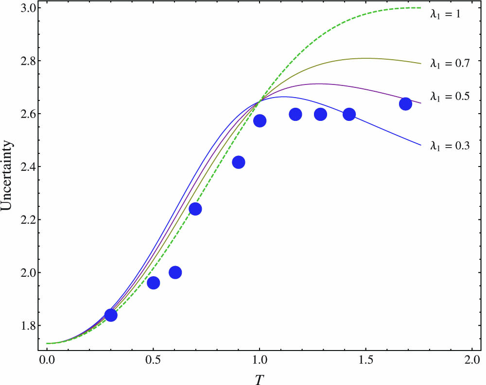
In the experiment^[18], a triphoton is produced by placing a pair of photons from Type II spontaneous parametric downconversion (SPDC) and a single photon from an attenuated laser (referred to as a local oscillator (LO)) into the same mode. The mixed light then goes through a variable partial polarizer (VPP), whose transmissivity ratio of the horizontal and the vertical mode photons is adjustable, and a quarter-wave plate (QWP) to get the desired state. The experimental data^[18] and theoretical curve of the uncertainty in ${\hat{S}}_{1}$ for the triphoton states is presented in Fig. 1. The dots indicate the experimental data points, while the curve represents the theoretical result calculated from the desired states. The calculation process is as follows.

Figure 1.Curves give uncertainty in ${\hat{S}}_{1}$ and $\sqrt{4 {(Δ {\hat{S}}_{1})}^{2}}$ as a function of $T (= T_{V} / T_{H})$ . The dashed line corresponds to the desired pure state, while the solid curves represent the mixed states with background terms taken into consideration. Different colors means different percentages of the desired state in the mixed state. The points represent Shalm’s experimental data^[18].

The polarization of a light field can be described by Stokes vectors ( $c = ℏ = 1$ )^[31]: ${\hat{S}}_{0} = \frac{1}{2} ({\hat{a}}_{H}^{†} {\hat{a}}_{H} + {\hat{a}}_{V}^{†} {\hat{a}}_{V}) = \frac{1}{2} ({\hat{n}}_{H} + {\hat{n}}_{V}), {\hat{S}}_{1} = \frac{1}{2} ({\hat{a}}_{H}^{†} {\hat{a}}_{H} - {\hat{a}}_{V}^{†} {\hat{a}}_{V}) = \frac{1}{2} ({\hat{n}}_{H} - {\hat{n}}_{V}), {\hat{S}}_{2} = \frac{1}{2} ({\hat{a}}_{H}^{†} {\hat{a}}_{V} + {\hat{a}}_{V}^{†} {\hat{a}}_{H}) = \frac{1}{2} ({\hat{n}}_{D} - {\hat{n}}_{A}), {\hat{S}}_{3} = \frac{1}{2} ({\hat{a}}_{H}^{†} {\hat{a}}_{V} - {\hat{a}}_{V}^{†} {\hat{a}}_{H}) = \frac{1}{2} ({\hat{n}}_{R} - {\hat{n}}_{L}),$ (1)where ${\hat{a}}_{H, V}$ and ${\hat{a}}_{H, V}^{†}$ are the annihilation and creation operators for the horizontal and vertical polarization modes, respectively. The vectors ${\hat{S}}_{1}$ , ${\hat{S}}_{2}$ and ${\hat{S}}_{3}$ obey SU(2) algebra: $[{\hat{S}}_{α}, {\hat{S}}_{β}] = i {\hat{S}}_{γ}$ with $α, β, γ \in {1,2, 3}$ . For a fixed photon number $N = 2 s$ , ${\hat{S}}^{2} = {\hat{S}}_{1}^{2} + {\hat{S}}_{2}^{2} + {\hat{S}}_{3}^{2} = s (s + 1)$ and ${\hat{S}}_{0} = s$ are invariant and commute with the other three Stokes operators. Following the standard theory of angular momentum, we choose eigenstates of ${\hat{S}}_{1}$ and $| s, n 〉 = {| s + n, s - n 〉}_{H, V}$ as the basis of the total Hilbert space, where the photon number states are defined as usual: ${| m, n 〉}_{H, V} = {(a_{H}^{†})}^{m} {(a_{V}^{†})}^{n} | 0 〉 / \sqrt{m! n!}$ . The SU(2) angular momentum states obey ${\hat{S}}_{\pm} | s, n 〉 = \sqrt{(s \mp n) (s \pm n + 1)} | s, n \pm 1 〉$ , with the ladder operators ${\hat{S}}_{\pm} = {\hat{S}}_{2} \pm i {\hat{S}}_{3}$ .

We might as well assume that the triphoton is performed by a pair of orthogonally polarized photons and a horizontally polarized single photon, which means that the input state of the VPP is $(a_{H}^{† 2} - a_{V}^{† 2}) a_{H}^{†} | 0 〉$ . After going through the VPP, the state is transformed into ${| ψ 〉}_{VPP} = T^{- {\hat{S}}_{1}} (a_{H}^{† 2} - a_{V}^{† 2}) a_{H}^{†} | 0 〉 = \frac{1}{\sqrt{3 + T^{4}}} (\sqrt{3} | \frac{3}{2}, \frac{3}{2} 〉 - T^{2} | \frac{3}{2}, - \frac{1}{2} 〉),$ (2)where $T = T_{V} / T_{H}$ denotes the transmissivity ratio of photons in the horizontal and vertical modes^[18]. After that, a QWP is adopted to rotate the polarization state into the basis of ${\hat{S}}_{3}$ , producing a new state^[30]: ${| ψ 〉}_{out} = x_{0} ({| 3,0 〉}_{H, V} - i {| 0,3 〉}_{H, V}) + y_{0} (i {| 2,1 〉}_{H, V} - {| 1,2 〉}_{H, V}),$ (3)where $x_{0} = \frac{1}{2} \sqrt{\frac{3}{2}} \frac{1 + T^{2}}{\sqrt{3 + T^{4}}}, y_{0} = \frac{1}{2 \sqrt{2}} \frac{3 - T^{2}}{\sqrt{3 + T^{4}}}$ .

The outcome is apparently a NOON state (one type of maximally entangled state): ${| ψ 〉}_{NOON} = \frac{\sqrt{2}}{2} ({| 3,0 〉}_{H, V} - i {| 0,3 〉}_{H, V})$ when $T = \sqrt{3}$ .

From Eq. (3), the spin fluctuation in ${\hat{S}}_{1}$ , i.e., the fluctuation of the difference between the photon number of two modes, can be calculated as follows: ${(Δ {\hat{S}}_{1})}^{2} = 〈 {\hat{S}}_{1}^{2} 〉 - {〈 {\hat{S}}_{1} 〉}^{2} = \frac{1}{2} (9 x_{0}^{2} + y_{0}^{2}) .$ (4)In the experiment^[18], the uncertainty in ${\hat{S}}_{1}$ is indicated by $\sqrt{4 {(Δ {\hat{S}}_{1})}^{2}}$ , which corresponds to the dashed curve in Fig. 1.

As we can see, the theoretical curve roughly matches the experimental results, but there is still room for improvement, especially when the value of $T$ is large. We suppose the error is due to the ignorance of the background terms during the calculation.

A triphoton is produced when a pair of photons from SPDC and a single photon from the LO are placed into the same mode. However, because ideal on-demand single-photon sources are not available, unwanted background events can occur, wherein the three detected photons may arise from a different combination of sources. According to Ref. [18], the desired state, which contains a pair of orthogonally polarized SPDC photons and an LO photon, has the highest probability to present in the mixed state (61.7% when $T = 1.7$ ). Among the background events, two states contribute the largest portion in probability, both of which are generated from three SPDC photons. For the sake of efficiency, only these two terms are accounted for the error presented in Fig. 1. These three events after VPP can be described as $| ψ_{1} 〉 = T^{- {\hat{S}}_{1}} \frac{1}{2 \sqrt{2}} {\hat{a}}_{H}^{†} ({\hat{a}}_{H}^{† 2} - {\hat{a}}_{V}^{† 2}) | 0 〉 = \frac{\sqrt{3} | \frac{3}{2}, \frac{3}{2} 〉 - T^{2} | \frac{3}{2}, - \frac{1}{2} 〉}{\sqrt{3 + T^{4}}}, | ψ_{2} 〉 = T^{- {\hat{S}}_{1}} \frac{1}{2 \sqrt{2}} ({\hat{a}}_{H}^{† 2} - {\hat{a}}_{V}^{† 2}) ({\hat{a}}_{H}^{†} + {\hat{a}}_{V}^{†}) | 0 〉 = \frac{\sqrt{3} | \frac{3}{2}, \frac{3}{2} 〉 + T | \frac{3}{2}, \frac{1}{2} 〉 - T^{2} | \frac{3}{2}, - \frac{1}{2} 〉 - \sqrt{3} T^{3} | \frac{3}{2}, - \frac{3}{2} 〉}{\sqrt{3 + T^{2} + T^{4} + 3 T^{6}}}, | ψ_{3} 〉 = T^{- {\hat{S}}_{1}} \frac{1}{2 \sqrt{2}} ({\hat{a}}_{H}^{† 2} - {\hat{a}}_{V}^{† 2}) ({\hat{a}}_{H}^{†} - {\hat{a}}_{V}^{†}) | 0 〉 = \frac{\sqrt{3} | \frac{3}{2}, \frac{3}{2} 〉 - T | \frac{3}{2}, \frac{1}{2} 〉 - T^{2} | \frac{3}{2}, - \frac{1}{2} 〉 + \sqrt{3} T^{3} | \frac{3}{2}, - \frac{3}{2} 〉}{\sqrt{3 + T^{2} + T^{4} + 3 T^{6}}},$ (5)where $| ψ_{1} 〉$ is the desired state, while $| ψ_{2} 〉$ and $| ψ_{3} 〉$ represent two background events. Since whether one background event will occur or not is independent, there should be no coherence between these three states, so we will only consider a mixed state whose density operator can be described as $\hat{ρ} = λ_{1} | ψ_{1} 〉 〈 ψ_{1} | + λ_{2} | ψ_{2} 〉 〈 ψ_{2} | + λ_{3} | ψ_{3} 〉 〈 ψ_{3} |,$ (6)where $λ_{1} + λ_{2} + λ_{3} = 1$ and $| ψ_{k} 〉 = a_{k} | \frac{3}{2}, \frac{3}{2} 〉 + b_{k} | \frac{3}{2}, \frac{1}{2} 〉 + c_{k} | \frac{3}{2}, - \frac{1}{2} 〉 + d_{k} | \frac{3}{2}, - \frac{3}{2} 〉$ for $k \in {1,2, 3}$ .

Next, we consider the photons passing through a QWP^[18], which can be described by a unitary operator $\exp (i π {\hat{S}}_{2} / 2)$ . Then we obtain ${\hat{ρ}}_{QWP} = e^{\frac{i π {\hat{S}}_{2}}{2}} \hat{ρ} e^{\frac{- i π {\hat{S}}_{2}}{2}} = λ_{1} | {\tilde{ψ}}_{1} 〉 〈 {\tilde{ψ}}_{1} | + λ_{2} | {\tilde{ψ}}_{2} 〉 〈 {\tilde{ψ}}_{2} | + λ_{3} | {\tilde{ψ}}_{3} 〉 〈 {\tilde{ψ}}_{3} |,$ (7) $| {\tilde{ψ}}_{k} 〉 = e^{\frac{i π {\hat{S}}_{2}}{2}} | ψ_{k} 〉 = x_{k} (| \frac{3}{2}, \frac{3}{2} 〉 - i | \frac{3}{2}, - \frac{3}{2} 〉) + y_{k} (i | \frac{3}{2}, \frac{1}{2} 〉 - | \frac{3}{2}, - \frac{1}{2} 〉),$ (8) $x_{k} = \frac{1}{2 \sqrt{2}} (a_{k} + i \sqrt{3} b_{k} - \sqrt{3} c_{k} - i d_{k}), y_{k} = \frac{1}{2 \sqrt{2}} (\sqrt{3} a_{k} - i b_{k} + c_{k} - i \sqrt{3} d_{k}) .$ (9)The spin fluctuation in ${\hat{S}}_{1}$ can be calculated as ${(Δ {\hat{S}}_{1})}^{2} = {〈 {\hat{S}}_{1} 〉}^{2} - 〈 {\hat{S}}_{1}^{2} 〉 = \sum_{k = 1}^{3} \frac{λ_{k}}{2} (9 {| x_{k} |}^{2} + {| y_{k} |}^{2}) .$ (10)By substituting Eq. (5) and Eq. (9) into Eq. (10), we obtain the function ${(Δ {\hat{S}}_{1})}^{2} = \frac{λ_{1} (7 T^{4} + 9 + 12 T^{2})}{4 T^{4} + 12} + \frac{(1 - λ_{1}) (9 T^{6} + 19 T^{4} + 9 + 19 T^{2})}{2 (T^{4} + 3 T^{6} + T^{2} + 3)} .$ (11)Now, we choose $λ_{1}$ as 30%, 50%, 70%, and 100% and plot the uncertainty in ${\hat{S}}_{1}$ , $\sqrt{4 {(Δ {\hat{S}}_{1})}^{2}}$ under these conditions in order to find a value that will fit the experimental data well. The results are shown in Fig. 1. We get the best result when $λ_{1} = λ_{2} + λ_{3} = 0.5$ . So we may take mixed states under this condition as the actual states. As one can see, after the background terms are taken into consideration properly, the theoretical curve matches the experimental data better, proving our assumption that the previous error is caused by background events.

Quantum metrology based upon maximally entangled NOON states results in super-resolving phase estimations^[11,12], showing that the QFI of maximally entangled states reaches the maximum. To calculate the QFI, we take the states as the input of a Mach–Zender interferometer, in which case $\hat{U} (ϕ) = e^{- i ϕ {\hat{S}}_{1}}$ . If we overlook the background terms, the QFI of the pure state ${| ψ 〉}_{out}$ in Eq. (3) can be calculated as^[20–22,24] $F_{Q} ({| ψ 〉}_{out}) = 4 {(Δ {\hat{S}}_{1})}^{2} = \frac{7 T^{4} + 9 + 12 T^{2}}{T^{4} + 3},$ (12)which reaches its peak value $F_{Q} {({| ψ 〉}_{out})}_{\max} = 9$ when $T = \sqrt{3}$ . Meanwhile, ${| ψ 〉}_{out}$ becomes a maximally entangled state ${| ψ 〉}_{NOON} = \frac{\sqrt{2}}{2} ({| 3,0 〉}_{H, V} - i {| 0,3 〉}_{H, V})$ under this circumstance. It can also be obtained that $F_{Q} {({| ψ 〉}_{out})}_{\min} = 3$ when $T = 0$ , and $F_{Q} ({| ψ 〉}_{out}) \to 7$ when $T \to \infty$ .

However, when the background terms are considered, the triphotons produced should be in a mixed state, reducing the maximal QFI. For the mixed states described by ${\hat{ρ}}_{QWP}$ in Eq. (7), the QFI can also be calculated. After a phase shift, this state becomes phase dependent^[32,33], described by its density operator $\hat{ρ} (ϕ) = e^{- i ϕ {\hat{S}}_{1}} {\hat{ρ}}_{QWP} e^{i ϕ {\hat{S}}_{1}} = \sum_{k = 1}^{3} λ_{k} | ψ_{k} (ϕ) 〉 〈 ψ_{k} (ϕ) |,$ (13) $| ψ_{k} (ϕ) 〉 = e^{- i ϕ {\hat{S}}_{1}} | {\tilde{ψ}}_{k} (ϕ) 〉 = A_{1 k} | \frac{3}{2}, \frac{3}{2} 〉 + A_{2 k} | \frac{3}{2}, \frac{1}{2} 〉 + A_{3 k} | \frac{3}{2}, - \frac{1}{2} 〉 + A_{4 k} | \frac{3}{2}, - \frac{3}{2} 〉,$ (14) $A_{1 k} = e^{- i \frac{3}{2} ϕ} x_{k}, A_{2 k} = i e^{- i \frac{1}{2} ϕ} x_{k}, A_{3 k} = - e^{i \frac{1}{2} ϕ} y_{k}, A_{4 k} = - i e^{i \frac{3}{2} ϕ} y_{k} .$ (15)To calculate the QFIs of mixed states, we here use the formula given in Ref. [19]: $F_{Q} = \sum_{m} \frac{{(\partial_{ϕ} ξ_{m} (ϕ))}^{2}}{ξ_{m} (ϕ)} + \sum_{m} ξ_{m} (ϕ) F_{Q, m} - \sum_{m, n}^{m \neq n} \frac{8 ξ_{m} (ϕ) ξ_{n} (ϕ)}{ξ_{m} (ϕ) + ξ_{n} (ϕ)} {| 〈 \partial_{ϕ} ξ_{m} (ϕ) | ξ_{n} (ϕ) 〉 |}^{2},$ (16)where $ξ (ϕ)$ and $| ξ (ϕ) 〉$ are respectively the eigenvalues and eigenstates of $\hat{ρ} (ϕ)$ , and $F_{Q, m} = 4 (〈 \partial_{ϕ} ξ_{m} (ϕ) | \partial_{ϕ} ξ_{m} (ϕ) 〉 - | 〈 \partial_{ϕ} ξ_{m} (ϕ) | ξ_{m} (ϕ) 〉 |^{2})$ (17)is the QFI of each eigenstate $| ξ_{m} (ϕ) 〉$ . To get the specific eigenstates of $\hat{ρ} (ϕ)$ , we can expand $\hat{ρ} (ϕ)$ as $\hat{ρ} (ϕ) = \sum_{k = 1}^{4} \sum_{l = 1}^{4} η_{k l} | \frac{3}{2}, \frac{5}{2} - k 〉 〈 \frac{3}{2}, \frac{5}{2} - l |,$ (18)with $η_{k l} = \sum_{j = 1}^{3} λ_{j} A_{k j} A_{l j}^{*}$ , which constructs a $4 \times 4$ matrix $η$ . Supposing that $| ξ_{m} (ϕ) 〉 = c_{1} | \frac{3}{2}, \frac{3}{2} 〉 + c_{2} | \frac{3}{2}, \frac{1}{2} 〉 + c_{3} | \frac{3}{2}, - \frac{1}{2} 〉 + c_{4} | \frac{3}{2}, - \frac{3}{2} 〉$ , we have the eigenvalue equation $η c = ξ c,$ (19)where $c = {(\begin{matrix} c_{1} & c_{2} & c_{3} & c_{4} \end{matrix})}^{T}$ .

After solving Eq. (19), we obtain $ξ (ϕ)$ and $| ξ (ϕ) 〉$ , and thus can calculate the QFI of the obtained triphoton states numerically. We here give a calculation example when $T$ approaches infinity. As previously mentioned, when $λ_{1} = λ_{2} + λ_{3} = 0.5$ , the mixed states are taken to be the actual states. By substituting $T \to \infty$ and $λ_{1} = λ_{2} + λ_{3} = 0.5$ into Eqs. (5), (6), (18) and (9), we can easily get $η = (\begin{matrix} 0.25 & 0.25 i e^{- i ϕ} & 0 & 0 \\ - 0.25 i e^{i ϕ} & 0.25 & 0 & 0 \\ 0 & 0 & 0.25 & - 0.25 i e^{- i ϕ} \\ 0 & 0 & 0.25 i e^{i ϕ} & 0.25 \end{matrix}),$ (20)and its two nonzero eigenvalues $ξ_{1} = ξ_{2} = 0.5$ , whose corresponding eigenvectors are $| ξ_{1} (ϕ) 〉 = \frac{\sqrt{2}}{2} i e^{- i \frac{3}{2} ϕ} | \frac{3}{2}, \frac{3}{2} 〉 + \frac{\sqrt{2}}{2} e^{- i \frac{1}{2} ϕ} | \frac{3}{2}, \frac{1}{2} 〉,$ (21) $| ξ_{2} (ϕ) 〉 = - \frac{\sqrt{2}}{2} i e^{i \frac{1}{2} ϕ} | \frac{3}{2}, - \frac{1}{2} 〉 + \frac{\sqrt{2}}{2} e^{i \frac{3}{2} ϕ} | \frac{3}{2}, - \frac{3}{2} 〉 .$ (22)Then we substitute the eigenvalues and eigenvectors into Eq. (16), and the QFI of the mixed states is calculated to be $F_{Q} {({\hat{ρ}}_{QWP})}_{T \to \infty} = 5$ . Similarly, we get $F_{Q} {({\hat{ρ}}_{QWP})}_{T \to 0} = 3$ .

Since the quantum Cramer–Rao bound of the uncertainty in a phase estimation satisfies the relation $δ ϕ_{CRB} = δ ϕ_{\min} = 1 / \sqrt{F_{Q}}$ , we can also numerically solve for $δ ϕ_{CRB}$ . The curve of $δ ϕ_{CRB}$ as a function of $T$ is shown in Fig. 2.

Figure 2.Curves give $δ_{CRB}$ as a function of $T$ . The red line corresponds to the desired pure state, while the blue one corresponds to the mixed state after considering background terms, when $λ_{1} = 0.5$ . The two filled dots represent the minimums of the two curves.

As shown in Fig. 2, the $δ ϕ_{CRB}$ of the mixed states comes to its minimum ${(δ ϕ_{CRB})}_{\min} = 0.369$ as $T = 1.28$ . The $δ ϕ_{CRB}$ of the mixed states is always less than the shot-noise limit $δ_{SNL} = 1 / \sqrt{3}$ , which is the largest value that could possibly be given by classical states. It is also found that the produced states have an obvious decline in phase estimations after considering the background states, as we presumed. To increase the QFI of the produced states and improve the estimation quality, the background events generated during the experiment should be suppressed.

In conclusion, we assume that the inconsistency of the theoretical curve with the experimental data is mainly because of ignorance of the background events. After taking two main background terms into consideration, we obtain a curve that matches better to the experiment. Then we calculate the QFI of the mixed states to evaluate its effect on the phase estimations, and find that its maximized QFI value is smaller than that of the desired NOON states, though still lager than ordinary, not-entangled states.

References

[1] Z. Y. Ou. Phys. Rev. A, 55, 2598(1997).

[2] H. Lee, P. Kok, J. P. Dowling. J. Mod. Opt., 49, 2325(2002).

[3] W. P. Bowen, R. Schnabel, H. A. Bachor, P. K. Lam. Phys. Rev. Lett., 88, 093601(2002).

[4] M. W. Mitchell, J. S. Lundeen, A. M. Steinberg. Nature, 429, 161(2004).

[5] X. Zhong, G. Lin, F. Zhou, Y. Niu, S. Gong. Chin. Opt. Lett., 13, 092701(2015).

[6] J. Qiu, G. Xiang, Y. Zhang, S. Han, Y. Gui. Chin. Opt. Lett., 12, 112701(2014).

[7] . Phys. Rev. A, 47, 5138(1993).

D. Leibfried, M. Kitagawa, M. Ueda, M. D. Barrett, T. Schaetz, J. Britton, J. Chiaverini, W. M. Itano, J. D. Jost, C. Langer, D. J. Wineland. Science, 304, 1476(2004).

[8] D. J. Wineland, J. J. Bollinger, W. M. Itano, D. J. Heinzen. Phys. Rev. A, 50, 67(1994).

[10] A. Sorensen, L.-M. Duan, J. I. Cirac, P. Zoller. Nature, 409, 63(2001).

[11] B. Yurke, S. L. McCall, J. R. Klauder. Phys. Rev. A, 33, 4033(1986).