
A. Praßelsperger, F. Balling, H.-P. Wieser, K. Parodi, J. Schreiber, "Ion-bunch energy acoustic tracing by modulation of the depth-dose curve," High Power Laser Sci. Eng. 11, 03000e42 (2023)
- High Power Laser Science and Engineering
- Vol. 11, Issue 3, 03000e42 (2023)
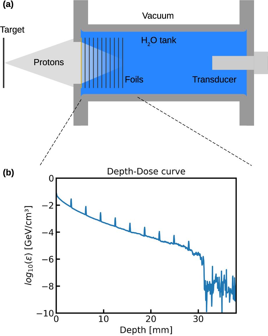
Fig. 1. (a) Schematic image of the new I-BEAT detector. It is placed within the centimeter range behind the laser target to capture most of the accelerated ions (shielding not shown). The ions deposit their energy along their propagation path until they stop within the water tank. In the lead modulator foils their electronic stopping power is increased to generate sharp energy density gradients. An exemplary integrated energy density curve versus depth for this setting is given in (b). Here a reference spectrum was used to simulate the 3D deposited energy distribution and, subsequently, the central x –z -plane was integrated along x to generate an axial (z ) plot. The stopping power ratio of the lead modulators compared with water is approximately 8.9.
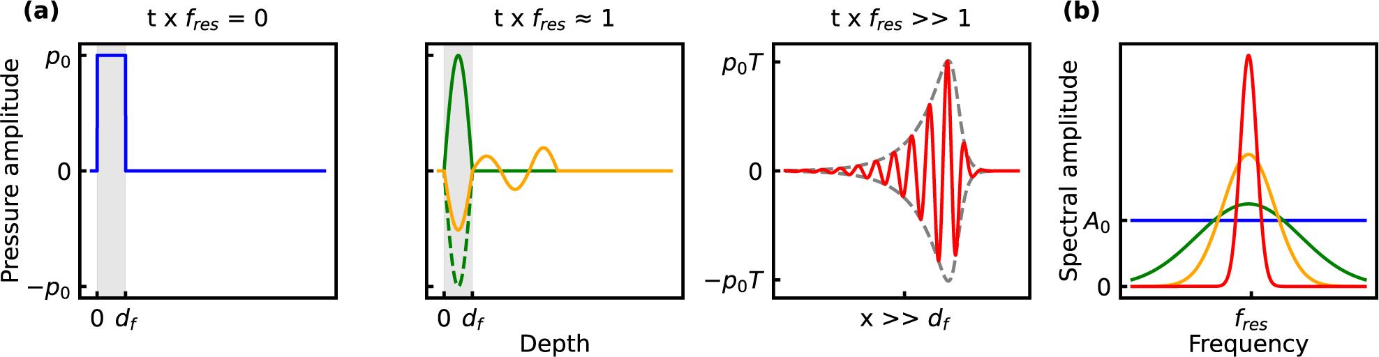
Fig. 2. (a) Temporal evolution of the initially sharp pressure gradients towards the resonance frequency. (b) Corresponding frequency spectra. The instantaneous pressure (blue,  ) shows steep gradients at the modulator foil (shaded region, thickness =
  ) interfaces corresponding to a broadband frequency spectrum. After the oscillation build-up, all off-resonant frequencies are canceled by destructive interference, and a standing wave (green,
  ) at resonance frequency, here
  , emerges. With each cycle a fraction of its amplitude, defined by the acoustic transmittance
  , is released into the medium as exemplified by the yellow curve (
 ). Thus, the spectrum narrows and the spectral amplitude (
 energy content) increases around the resonance frequency. Overall, a pulse train is emitted by the modulator characterized by an envelope (gray dashed) with a build-up function fitted as
  , which is defined by the modulator’s 3D extent and a ring-down function
  depending on the material’s acoustic reflectivity,
  . The characteristic times
  and
and  specify the signal’s rise and decay time, respectively. The entire modulator signal (red)
  is thus given by
  with
with  and a carrier frequency of
  .
.
) shows steep gradients at the modulator foil (shaded region, thickness = ) interfaces corresponding to a broadband frequency spectrum. After the oscillation build-up, all off-resonant frequencies are canceled by destructive interference, and a standing wave (green, ) at resonance frequency, here , emerges. With each cycle a fraction of its amplitude, defined by the acoustic transmittance , is released into the medium as exemplified by the yellow curve (). Thus, the spectrum narrows and the spectral amplitude ( energy content) increases around the resonance frequency. Overall, a pulse train is emitted by the modulator characterized by an envelope (gray dashed) with a build-up function fitted as , which is defined by the modulator’s 3D extent and a ring-down function depending on the material’s acoustic reflectivity, . The characteristic times and specify the signal’s rise and decay time, respectively. The entire modulator signal (red) is thus given by with and a carrier frequency of . Fig. 3. Simulated pressure trace of the energy distribution shown in Figure 1(b) . In (a) the temporal profile shows the 10 individual modulator pulse trains starting at 46 μs with a spacing of 2 μs (blue). The dashed lines show the onset of the individual foil signals and their corresponding depths with respect to the entrance window. At 67 μs the window signal (EW) is overlapping the pulse of the last modulator. Note that the individual pulses are temporally delayed due to the signals rise times (see Figure 2 ). For reference, the inset shows the logarithmic signal for a water reservoir without any modulators (orange). (b) The corresponding Fourier-transformed spectra of the pressure traces. In the modulated signal three prominent characteristics can be distinguished. The resonant signals from the entrance window and the modulators manifest in the peaks at 9.8 and 19.6 MHz, that is, the first two resonant modes. A low-frequency (DC) component ( MHz) emitted by the overall spread-out energy deposition region and defined by wavelengths much larger than the foil thickness is also registered as these low frequencies penetrate the modulators unperturbed. The entire signal is superimposed with a frequency modulation defined by the foil spacing. Compared with the unmodulated reference case, the spectral amplitude in the first modulation mode is completely maintained.
MHz) emitted by the overall spread-out energy deposition region and defined by wavelengths much larger than the foil thickness is also registered as these low frequencies penetrate the modulators unperturbed. The entire signal is superimposed with a frequency modulation defined by the foil spacing. Compared with the unmodulated reference case, the spectral amplitude in the first modulation mode is completely maintained. Fig. 4. In (a) the energy density reconstruction  for an SNR of
  without filtering is plotted. The relative error to the input
  is below
  . (b) The ratio
  versus the normal SNR for each source foil. For SNR values around 1 the curves start to diverge due to the reconstruction starting to predominantly minimize on the noise signal. A better performance can be observed for temporally more peaked signals originating from deeper modulators. The performance of the reconstruction with Gaussian frequency filtering around
  with an FWHM of 2 MHz is shown in (c). It is improved by
  in SNR values as a result of the reduction in noise while simultaneously maintaining the main signal. The performance is better for temporally longer signals, most likely caused by an overestimation of the envelope function used for reconstruction (see
 Equation (2) ) due to resonant noise, yielding a worse result for temporally shorter signals.
for an SNR of without filtering is plotted. The relative error to the input is below . (b) The ratio versus the normal SNR for each source foil. For SNR values around 1 the curves start to diverge due to the reconstruction starting to predominantly minimize on the noise signal. A better performance can be observed for temporally more peaked signals originating from deeper modulators. The performance of the reconstruction with Gaussian frequency filtering around with an FWHM of 2 MHz is shown in (c). It is improved by in SNR values as a result of the reduction in noise while simultaneously maintaining the main signal. The performance is better for temporally longer signals, most likely caused by an overestimation of the envelope function used for reconstruction (see 

Set citation alerts for the article
Please enter your email address

© Copyright 2018-2021 | Chinese Laser Press. All Rights Reserved 沪ICP备15018463号-20