
A. Praßelsperger, F. Balling, H.-P. Wieser, K. Parodi, J. Schreiber, "Ion-bunch energy acoustic tracing by modulation of the depth-dose curve," High Power Laser Sci. Eng. 11, 03000e42 (2023)
- High Power Laser Science and Engineering
- Vol. 11, Issue 3, 03000e42 (2023)
Abstract
1 Introduction
Since the advent of laser-ion acceleration in 2000, the field has been steadily progressing[1–4]. While previously ions were accelerated predominantly by target normal sheath acceleration (TNSA) to up to tens of MeV, state-of-the-art PW systems with improved temporal laser contrast reach new acceleration regimes. As such, radiation pressure acceleration and relativistic-induced transparency accelerate ions within sub-ps laser–plasma interactions, resulting in pronounced angular emission characteristics[5]. At these acceleration parameters, protons approaching the 100 MeV kinetic energy barrier as well as carbon ions exceeding 80 MeV/u have been observed[6–8]. With improving parameters of this technique, the number of applications is increasing steadily. As such, the first radio-biological in vivo studies of tumor irradiation with laser-accelerated ions investigating the FLASH effect have been conducted[9], fundamental ion–matter interactions in high-energy deposition regions have been investigated[10–12] and the application of laser-accelerated ion bunches for fuel ignition in inertial confinement fusion has been discussed[13–15]. All of these applications require a precise ion spectrum determination for depth–dose verification, model input and cross-section maximization. Peak beam currents exceeding mega-amperes pose challenges to detectors applied for spectral measurements[16]. The harsh conditions encountered, especially in the aperture angle close to the laser–plasma interaction where strong electro-magnetic pulses (EMPs) disturb (or even damage) electronics, prevent the application of complementary metal oxide semiconductor (CMOS) detectors, such as RadEyes[17,18]. On the other hand, when measuring further downstream of the laser–plasma interaction as, for example, done by Thomson parabolas, angular emission features such as energy-dependent cone narrowing are forfeited[19,20]. Other non-invasive detection modalities, such as integrating current transformers, measure the total beam charge without a precise spectrum reconstruction[21]. Due to these issues, non-electronic methods such as radio chromic films (RCFs) or Columbia Resin #39 (CR39) are still utilized as widespread standard ion diagnostics in laser-ion-acceleration experiments[22,23]. They suffer from none of the discussed drawbacks, but nevertheless they do not allow for online read-out. Particularly for highly energetic particles exceeding 100 MeV, the RCF stacks used in experiments can become quite thick and evaluation is tedious.
A rather new approach for energy density determination of laser-accelerated particles is ionoacoustics[24]. It capitalizes on the measurement of the ultrasound wave emitted by the heat-expansion of a medium when energy is deposited by ions in a short amount of time[25,26]. The pressure trace
The ion-bunch energy acoustic tracing (I-BEAT) detector measures this far-field pressure trace on a single-shot to reconstruct the initial energy deposition and the corresponding particle spectrum down to a minimum of
Sign up for High Power Laser Science and Engineering TOC. Get the latest issue of High Power Laser Science and Engineering delivered right to you!Sign up now
Demonstrated by several experiments, this ionoacoustic approach is also capable of detecting mono-energetic bunches of 20 MeV protons down to minimum energy deposition of
Adversely, the inherent drawback of this method is the reliance on a spatial energy density gradient to produce the pressure amplitude. This gradient is induced by the Bragg-peak for mono-energetic ion beams. Laser-accelerated ion beams, however, typically exhibit an exponential ion energy spectrum with certain additional features, depending on the acceleration regime[1,5,7]. These spectra range over orders of magnitude and the corresponding energy densities deposited in matter are typically dominated by the low-energy particles. Therefore, the dynamic range of ionoacoustic measurements often is insufficient to measure and reconstruct the entire spectrum and is sensitive only to their low-energetic components[27,32].
Here we present a simulation study of a new version of I-BEAT, solving this problem by artificially introducing gradients to the energy density distribution, that is, tracing ionoacoustic modulations of broad energy distributions (TIMBRE). The detector is designed to be placed within a few centimeter range behind the target to collect the majority of the accelerated particles. Similar to the spherical ionoacoustic waves with resonant frequency (SPIRE) technique[33,34], we use special modulator foils to increase the electronic stopping power of the ions. This generates high-energy density gradients at the water–modulator interfaces and, hence, strong broadband frequency signals. In addition, placing the modulator foils equidistantly results in particularly strong resonant waves, allowing for reconstruction of the energy deposited in the modulator foils. This overcomes theoretical predictions of minimum detection thresholds of the Bragg-peak, given that media interfaces are spatially more pronounced in their electronic stopping gradients[35].
2 Detector concept
2.1 Modulator foils
Figure 1(a) shows a cross-section scheme of the detector. It consists of a vacuum-compatible water tank that is placed within the centimeter range behind the laser target to collect most of the accelerated ions. A Kapton entrance window is used for the ions to enter the water volume. Inside the tank, multiple flat foils act as modulators to shape the dose distribution. By this method, spatially separated energy density distribution characteristics are encoded in the acoustic source signal. To find an optimal modulator material four quantities were optimized. First, the ion stopping power in the modulators should be high compared with water to generate large energy density gradients at the interfaces. Second, the modulator’s Grüneisen parameter
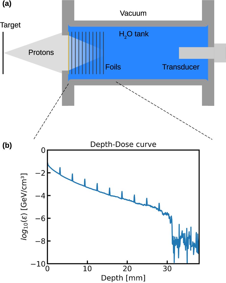
Figure 1.(a) Schematic image of the new I-BEAT detector. It is placed within the centimeter range behind the laser target to capture most of the accelerated ions (shielding not shown). The ions deposit their energy along their propagation path until they stop within the water tank. In the lead modulator foils their electronic stopping power is increased to generate sharp energy density gradients. An exemplary integrated energy density curve versus depth for this setting is given in (b). Here a reference spectrum was used to simulate the 3D deposited energy distribution and, subsequently, the central
2.2 Signal generation and propagation
In Figure 2, the process of the pressure wave generation is shown. The initial pressure has a step gradient at the modulator interfaces, which comes with a wide frequency bandwidth in Fourier space. Off-resonant components of this frequency band interfere destructively in subsequent oscillations and frequencies close to the resonance
![]()
Figure 2.(a) Temporal evolution of the initially sharp pressure gradients towards the resonance frequency. (b) Corresponding frequency spectra. The instantaneous pressure (blue,  ) shows steep gradients at the modulator foil (shaded region, thickness =
  ) interfaces corresponding to a broadband frequency spectrum. After the oscillation build-up, all off-resonant frequencies are canceled by destructive interference, and a standing wave (green,
  ) at resonance frequency, here
  , emerges. With each cycle a fraction of its amplitude, defined by the acoustic transmittance
  , is released into the medium as exemplified by the yellow curve (
 ). Thus, the spectrum narrows and the spectral amplitude (
 energy content) increases around the resonance frequency. Overall, a pulse train is emitted by the modulator characterized by an envelope (gray dashed) with a build-up function fitted as
  , which is defined by the modulator’s 3D extent and a ring-down function
  depending on the material’s acoustic reflectivity,
  . The characteristic times
  and
and  specify the signal’s rise and decay time, respectively. The entire modulator signal (red)
  is thus given by
  with
with  and a carrier frequency of
  .
.
Transmitting through a subsequent modulator foil will only weakly reduce the spectral amplitude of the pulse trains. This is due to the phase difference of the pulse train’s jth wave-cycle reflection
3 Methods
For all simulations a reference differential TNSA angular and energy proton spectrum with a maximum energy of 60 MeV was assumed[32]. Both energy and angular distributions were included in a FLUKA source file to calculate the energy distribution in the detector[36,37]. The detector was placed 6 cm behind the particle source. Considering the 1.7 cm thickness of the front flange, this defines the source to entrance window distance as 7.7 cm. The entire detector was modeled as shown in Figure 1(a), with an additional 2 cm thick plastic shielding (entrance window spared) and a 15 μm thick aluminum foil in front of the flange, to stop all ions of kinetic energies below approximately 2 MeV and reduce background noise by energy deposited in the detector’s casing.
Subsequently, the geometry and the deposited energy data were exported to a k-wave code to simulate the resulting pressure evolution within the detector using the deposition data according to Equation (1) as the source[38–40]. For pressure measurement, an Olympus Videoscan V311-SU transducer with a resonance frequency of 10 MHz was modeled, while its electrical impulse response function was neglected.
For the reconstruction of the energy density from a pressure trace, a semi-3D algorithm was specially designed. It requires only the geometry and a measured pressure trace
The average reconstruction time of a depth–dose profile scales linearly with the temporal window that is considered for the isolated signals
4 Results
Figure 3(a) presents the pressure trace
![]()
Figure 3.Simulated pressure trace of the energy distribution shown in  MHz) emitted by the overall spread-out energy deposition region and defined by wavelengths much larger than the foil thickness is also registered as these low frequencies penetrate the modulators unperturbed. The entire signal is superimposed with a frequency modulation defined by the foil spacing. Compared with the unmodulated reference case, the spectral amplitude in the first modulation mode is completely maintained.
Comparing both traces in Figure 3, modulated and unmodulated, shows the inherent asset of this detector approach. In the temporal traces it can be seen that the dynamic range in the unmodulated case (orange) is more than
Figure 4(a) shows the energy density reconstructed from the modulated pressure trace in Figure 3 with an SNR of
![]()
Figure 4.In (a) the energy density reconstruction  for an SNR of
  without filtering is plotted. The relative error to the input
  is below
  . (b) The ratio
  versus the normal SNR for each source foil. For SNR values around 1 the curves start to diverge due to the reconstruction starting to predominantly minimize on the noise signal. A better performance can be observed for temporally more peaked signals originating from deeper modulators. The performance of the reconstruction with Gaussian frequency filtering around
  with an FWHM of 2 MHz is shown in (c). It is improved by
  in SNR values as a result of the reduction in noise while simultaneously maintaining the main signal. The performance is better for temporally longer signals, most likely caused by an overestimation of the envelope function used for reconstruction (see
The assignment of a reconstructed energy density to a specific modulator foil limits the spatial resolution to the thickness of this foil, that is, 100 μm, which is similar to what an integrated RCF stack provides. However, the intermediate signal originating from in between foils cannot be reconstructed. Stacking modulators closer and increasing their number will shift the
5 Conclusion
The simulation study suggests that TIMBRE is capable of measuring broadband, laser-accelerated ion bunches. The increased energy density gradient and the enhancement at the resonance frequency due to the modulation of the water reservoir increase the sensitivity by at least
In particular, due to its capability of immediate feedback and simplicity, we expect the presented detector approach to become a valuable addition to other diagnostics, if not a primary ion diagnostic for laser–plasma-based ion sources, once tested extensively in experiments.
References
[1] R. A. Snavely, M. H. Key, S. P. Hatchettand, T. E. Cowan, M. Roth, T. W. Phillips, M. A. Stoyer, E. A. Henry, T. C. Sangster, M. S. Singh, S. C. Wilks, A. MacKinnon, A. Offenberger, D. M. Pennington, K. Yasuike, A. B. Langdon, B. F. Lasinski, J. Johnson, M. D. Perry, E. M. Campbell. Phys. Rev. Lett., 85, 2945(2000).
[2] E. L. Clark, K. Krushelnick, J. R. Davies, M. Zepf, M. Tatarakis, F. N. Beg, A. Machacek, P. A. Norreys, M. I. K. Santala, I. Watts, A. E. Dangor. Phys. Rev. Lett., 84, 670(2000).
[3] A. Maksimchuk, S. Gu, K. Flippo, D. Umstadter, V. Y. Bychenkov. Phys. Rev. Lett., 84, 4108(2000).
[4] J. Schreiber, P. R. Bolton, K. Parodi. Revi. Sci. Instrum., 87, 071101(2016).
[5] S. Keppler, N. Elkina, G. A. Becker, J. Hein, M. Hornung, M. Mäusezahl, C. Rödel, I. Tamer, M. Zepf, M. C. Kaluza. Phys. Rev. Res., 4, 013065(2022).
[6] F. Wagner, O. Deppert, C. Brabetz, P. Fiala, A. Kleinschmidt, P. Poth, V. A. Schanz, A. Tebartz, B. Zielbauer, M. Roth, T. Stöhlker, V. Bagnoud. Phys. Rev. Lett., 116, 205002(2016).
[7] A. Higginson, R. J. Gray, M. King, R. J. Dance, S. D. R. Williamson, N. M. H. Butler, R. Wilson, R. Capdessus, C. Armstrong, J. S. Green, S. J. Hawkes, P. Martin, W. Q. Wei, S. R. Mirfayzi, X. H. Yuan, S. Kar, M. Borghesi, R. J. Clarke, D. Neely, P. McKenna. Nat. Commun., 9, 724(2018).
[8] D. Jung, L. Yin, J. Albright, D. C. Gautier, S. Letzring, B. Dromey, M. Yeung, R. Hörlein, R. Shah, S. Palaniyappan. New J. Phys., 15, 023007(2013).
[9] F. Kroll, F.-E. Brack, C. Bernert, S. Bock, E. Bodenstein, K. Brüchner, T. E. Cowan, L. Gaus, R. Gebhardt, U. Helbig, L. Karsch, T. Kluge, S. Kraft, M. Krause, E. Lessmann, U. Masood, S. Meister, J. Metzkes-Ng, A. Nossula, J. Pawelke, J. Pietzsch, T. Püschel, M. Reimold, M. Rehwald, C. Richter, H.-P. Schlenvoigt, U. Schramm, M. E. P. Umlandt, T. Ziegler, K. Zeil, E. Beyreuther. Nat. Phys., 18, 316(2022).
[10] B. Dromey, M. Coughlan, L. Senje, M. Taylor, S. Kuschel, B. Villagomez-Bernabe, R. Stefanuik, G. Nersisyan, L. Stella, J. Kohanoff, M. Borghesi, F. Currell, D. Riley, D. Jung, C.-G. Wahlström, C. L. S. Lewis, M. Zepf. Nat. Commun., 7, 10642(2016).
[11] M. Taylor, M. Coughlan, G. Nersisyan, L. Senje, D. Jung, F. Currell, D. Riley, C. L. S. Lewis, M. Zepf, B. Dromey. Plasma Phys. Control. Fusion, 60, 054004(2018).
[12] A. Prasselsperger, M. Coughlan, N. Breslin, M. Yeung, C. Arthur, H. Donnelly, S. White, M. Afshari, M. Speicher, R. Yang, B. Villagomez-Bernabe, F. J. Currell, J. Schreiber, B. Dromey. Phys. Rev. Lett., 127, 186001(2021).
[13] M. Roth, T. E. Cowan, M. H. Key, S. P. Hatchett, C. Brown, W. Fountain, J. Johnson, D. M. Pennington, R. A. Snavely, S. C. Wilks, K. Yasuike, H. Ruhl, F. Pegoraro, S. V. Bulanov, E. M. Campbell, M. D. Perry, H. Powell. Phys. Rev. Lett., 86, 436(2001).
[14] J. Badziak, J. Domanski. Nucl. Fusion, 61, 046011(2021).
[15] J. Badziak, J. Domanski. Nucl. Fusion, 62, 086040(2022).
[16] M. Borghesi. Nucl. Instrum. Methods Phys. Res. A, 740, 6(2014).
[17] F. H. Lindner, J. H. Bin, F. Englbrecht, D. Haffa, P. R. Bolton, Y. Gao, J. Hartmann, P. Hilz, C. Kreuzer, T. M. Ostermayr, T. F. Rösch, M. Speicher, K. Parodi, P. G. Thirolf, J. Schreiber. Rev. Sci. Instrum., 89, 013301(2018).
[18] S. Reinhardt, C. Granja, F. Krejci, W. Assmann. J. Instrum., 6, C12030(2011).
[19] K. Harres, M. Schollmeier, E. Brambrink, P. Audebert, A. Blazevic, K. Flippo, D. C. Gautier, M. Geißel, B. M. Hegelich, F. Nürnberg, J. Schreiber, H. Wahl, M. Roth. Rev. Sci. Instrum., 79, 093306(2008).
[20] D. C. Carroll, P. Brummitt, D. Neely, F. Lindau, O. Lundh, C.-G. Wahlström, P. McKenna. Nucl. Instrum. Methods Phys. Res. Sect. A, 620, 23(2010).
[21] L. D. Geulig, L. Obst-Huebl, K. Nakamura, J. Bin, Q. Ji, S. Steinke, A. M. Snijders, J.-H. Mao, E. A. Blakely, A. J. Gonsalves, S. Bulanov, J. van Tilborg, C. B. Schroeder, C. G. R. Geddes, E. Esarey, M. Roth, T. Schenkel. Rev. Sci. Instrum., 93, 103301(2022).
[22] W. L. McLaughlin, Y.-D. Chen, C. G. Soares, A. Miller, G. Van Dyk, D. F. Lewis. Nucl. Instrum. Methods Phys. Res. Sect. A, 1, 165(1991).
[23] R. M. Cassou, E. V. Benton. Nucl. Track Detection, 2, 173(1978).
[24] K. Parodi, W. Assmann. Mod. Phys. Lett. A, 30, 1540025(2015).
[25] L. Sulak, T. Armstrong, H. Baranger, M. Bregman, M. Levi, D. Mael, J. Strait, T. Bowen, A. E. Pifer, P. A. Polakos, H. Bradner, A. Parvulescu, W. V. Jones, J. Learned. Nucl. Instrum. Methods, 161, 203(1979).
[26] G. A. Askariyan, B. A. Dolgoshein, A. N. Kalinovsky, N. V. Mokhov. Nucl. Instrum. Methods, 164, 267(1979).
[27] D. Haffa, R. Yang, J. Bin, S. Lehrack, F. Brack, H. Ding, F. S. Englbrecht, Y. Gao, J. Gebhard, M. Gilljohann, J. Götzfried, J. Hartmann, S. Herr, P. Hilz, S. D. Kraft, C. Kreuzer, F. Kroll, F. H. Lindner, J. Metzkes-Ng, T. M. Ostermayr, E. Ridente, T. F. Rösch, G. Schilling, H.-P. Schlenvoigt, M. Speicher, D. Tarayand, M. Würl, K. Zeil, U. Schramm, S. Karsch, K. Parodi, P. R. Bolton, W. Assmann, J. Schreiber. Sci. Rep., 9, 6714(2019).
[28] W. Assmann, S. Kellnberger, S. Reinhardt, S. Lehrack, A. Edlich, P. G. Thirolf, M. Moser, G. Dollinger, M. Omar, V. Ntziachristos, K. Parodi. J. Med. Phys., 42, 567(2015).
[29] S. Lehrack, W. Assmann, M. Bender, D. Severin, C. Trautmann, J. Schreiber, K. Parodi. Nucl. Instrum. Methods Phys. Res. A, 950, 162935(2020).
[30] S. Lehrack, W. Assmann, D. Bertrand, S. Henrotin, J. Herault, V. Heymans, F. Vander Stappen, P. G Thirolf, M. Vidal, J. Van de Walle, K. Parod. Phys. Med. Biol., 62, L20(2017).
[31] S. Kellnberger, W. Assmann, S. Lehrack, S. Reinhardt, P. G. Thirolf, D. Queiros, G. Sergiadis, G. Dollinger, K. Parodi, V. Ntziachristos. Sci. Rep., 6, 29305(2016).
[32] F. Balling, S. Gerlach, A.-K. Schmidt, V. Bagnoud, J. Hornung, B. Zielbauer, K. Parodi, J. Schreiber, 11779, 117790T(2021).
[33] T. Takayanagi, T. Uesaka, M. Kitaoka, M. B. Unlu, K. Umegaki, H. Shirato, L. Xing, T. Matsuura. Sci. Rep., 9, 4011(2019).
[34] T. Takayanagi, T. Uesaka, Y. Nakamura, M. B. Unlu, Y. Kuriyama, T. Uesugi, Y. Ishi, N. Kudo, M. Kobayashi, K. Umegaki, S. Tomioka, T. Matsuura. Sci. Rep., 10, 20385(2020).
[35] M. Ahmad, L. Xiang, S. Yousefi, L. Xing. Med. Phys., 42, 5735(2015).
[36] A. Ferrari, J. Ranft, P. R. Sala, A. Fasso. Fluka: A Multiparticle Transport Code(2005).
[37] T. T. Böhlen, F. Cerutti, M. P. W. Chin, A. Fasso, A. Ferrari, P. G. Ortega, A. Mairani, P. R. Sala, G. Smirnov, V. Vlachoudis. Nucl. Data Sheets, 120, 211(2014).
[38] B. E. Treeby, B. T. Cox. J. Biomed. Opt., 15, 021314(2010).
[39] B. E. Treeby, B. T. Cox. J. Acoust. Soc. Am., 127, 2741(2010).
[40] B. E. Treeby, J. Jaros, A. P. Rendell, B. T. Cox. J. Acoust. Soc. Am., 131, 4324(2012).


Set citation alerts for the article
Please enter your email address

© Copyright 2018-2021 | Chinese Laser Press. All Rights Reserved 沪ICP备15018463号-20