Edge enhancement is uniquely important as perception of edge is a key factor for the human visual system to identify or comprehend the contents of an image. It has vital roles in broad applications, such as increasing discrimination capacity in pattern recognition [1], detecting dislocation of crystal in biological cells [2], and identifying lesion boundaries of cancer [3–6]. The realization of edge enhancement can be traced back to Zernike’s seminal work [7], where the phase or intensity gradient of an object is enhanced for conspicuity strengthening and tiny-feature detection. Nowadays, edge enhancement can be accomplished digitally through signal processing methods, such as spatial differentiation [8], wavelet transform [9], and Hilbert transform [10], or through physical settings. One well-known example is spiral phase contrast (SPC) imaging, where a spiral phase plate with a topological charge l=1 is placed in the Fourier plane of a 4f system [11–13]. Due to the peculiar symmetry of spiral phase, gradients of the phase and intensity profile can be isotropically enhanced. The SPC method was later extended for microscopy to make image brightness and contrast significantly better than conventional versions [14]. Another strategy is to employ the photorefractive effect to highlight the edge information of an intensity pattern [15–17]. Responding to the interferogram, photorefractive materials, governed by the four-wave-mixing mechanism [15], form a volumetric optical grating with different local diffraction efficiencies. Manipulating such gratings may maximize the diffraction efficiency for edges only while minimizing that for other parts; consequentially, the boundaries of the pattern are enhanced [15]. In addition, some physical filters, such as the Laguerre–Gaussian spatial filter [18] and Airy spiral phase filter [19], are also developed to achieve high contrast edge enhancement.

While promising, all filters mentioned above, no matter digital or physical, can only perform edge detection in free space or process signals obtained with ballistic or quasi-ballistic light. These approaches are not able or have not been verified to be compatible with strong scattering media (e.g., ∼1mm beneath human skin [20]), when photons are multiply scattered and optical information is completely disordered [21]. Therefore, existing edge enhancement methods encounter the same trade-off between penetration depth and resolution as all other biomedical optical techniques [22]. High-resolution edge information processing and retrieval at depths in scattering media have been desired in many optical applications that yet remain unexplored.

This study aims to tackle this challenge from the perspective of optical wavefront shaping, a relatively new field conceived to manipulate scattered light beyond the diffusion limit [23–27]. Optical phase conjugation (OPC) [24,27–29] is an example of wavefront shaping that exploits the bilateral nature of a light trajectory to “time-reverse” scattered light [30]. The execution of OPC requires an analog [27,31] or digital [28,29,32,33] phase conjugation mirror (PCM) that, first, holographically records the phase profile of scattered light and, second, projects its phase-conjugated copy back to the medium. As a result, the intensity profile of the original incident light field before being scattered can be reconstructed. The whole procedure can be accomplished with two or three steps [33], achieving light manipulation through turbidity as rapidly as a few milliseconds [34,35]. While related, such a capability thus far has not yet been extended for edge enhancement through scattering media. In this study, we take inspiration from the classic photorefractive approach for edge enhancement in free space [15], and develop a digital optical phase conjugation (DOPC) setup to achieve robust and tunable time-reversed speckle suppression and edge enhancement through thick scattering media by a two-step procedure. First, a hologram that accurately encodes the information of the edge only is recorded. Second, the edge pattern is selectively decoded by phase conjugating the scattered light. The proposed method is demonstrated experimentally with scalable edge enhancement performance out of seemingly random speckle patterns. Although a lot needs to be furthered, this work potentially can be of instructive significance to the processing, comprehension, and analysis of optical images with the presence of scattering.

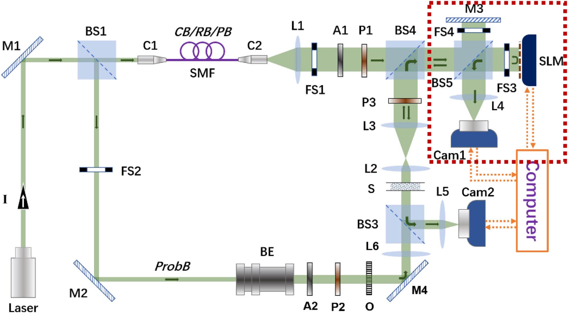
The configuration of the DOPC system is presented in Fig. 1. A CW laser source (EXLSR-532–200-CDRH, Spectra Physics, coherence length=300m) emits a laser beam (λ=532nm), which is split by a beam splitter cube (BS1) into two arms. One is probe beam, and the other is multifunctional beam (calibration/reference/playback beam). The probe beam is expanded by a collimated beam expander, and its intensity profile is shaped by a 1951 USAF resolution test chart (Edmund Optics Inc.). The image of the resolution test chart is relayed onto the interior surface of a diffuser (600 grit polished, Thorlabs) by L6. On the other side, the multifunctional beam is spatially shaped by a single-mode fiber (HP-532, Thorlabs, 1 m long) to mimic a quasi-ideal point source at the exit of the collimator (C2). The beam is expanded by a best-form lens (L1) before entering the digital PCM module. At the beam splitter cube (BS4), the probe beam and the multipurpose beam merge and are relayed together to the digital PCM, which is configurated by the combination of a scientific complementary metal–oxide semiconductor camera (sCMOS; pco.edge 5.5; PCO; pixel size, 6.5μm×6.5μm) and a phase-only spatial light modulator (SLM, PLUTO-VIS-056, HOLOEYE). The SLM and the sCMOS camera are pixel-to-pixel conjugated to each other, with a misalignment error less than 1 pixel. The diffused light pattern right after the diffuser is imaged on the plane of SLM through a 4f system configured by L2 and L3, where the diffuser and the plane of SLM are spatially quasi-conjugated with each other. The digital PCM has two main purposes, hologram recording and playback, which are, respectively, accomplished by the sCMOS camera and the phase-only SLM. To observe the playback wavefront, another CMOS camera (Cam2; pixel size, 2.5μm×2.5μm) and L5 are employed to image the reconstructed intensity distribution of the playback beam after transmitting through the turbid sample. Polarizations and intensities of the probe beam and the multipurpose beam are adjusted by two linear polarizers (P1 and P2) and neutral-density attenuators (A1 and A2), respectively. Four fast shutters (FS1−4) are equipped to control the ON or OFF state of light beams. Detailed procedures of the DOPC operation can be referred to Refs. [32,33].

A former study has demonstrated how edges of a binary pattern can be enhanced in free space via the photorefractive effect with a piece of BaTiO3 photorefractive crystal [15]. The method proposed in this work is actually a digital analogue of the aforementioned photorefractive edge enhancer. Functions of the photorefractive crystal are provided by a digital PCM, a spatially conjugated camera-SLM module, as enclosed by the red dashed line in Fig. 1. On one hand, holographic information is recorded digitally using a digital camera (Cam1, Fig. 1); on the other hand, an SLM is able to create variable phase profiles, mimicking the effect of grating with variable diffraction efficiency in the crystal.

Starting with hologram recording, the working principles of DOPC-based edge enhancement can be explained as below. The hologram recorded by Cam1 can be written as where Ih, Iref, and Iprob denote the intensity of hologram, the reference beam, and the probe beam, respectively; φ is the phase difference between the reference beam and the probe beam. The local modulation efficiency (M.E.) of PCM, determined by contrast of the hologram recorded by Cam1, can be expressed as It can be seen that the local M.E. of PCM is dominated by the modulation depth (MD=2Iprob·IrefIprob+Iref) [15]. This term can be expressed as a function of the intensity ratio of the probe and reference beams, i.e., r=IprobIref, so that MD(r)=2r1+r. As a result, M.E. can be written as M.E.=1+MD(r)·cosφ. Considering the one-dimensional situation as follows without scattering media: where a, b, and m are three finite constants. It represents a simple case of a hologram written to Cam1, where the reference beam is of uniform intensity while the probe beam is of a binary intensity profile, i.e., a box function with a width of m, symmetrical with respect to the origin. But, there is an extreme condition for this situation, that is the intensity of the probe beam is considerably larger than that of the reference beam, i.e., a≪b. For the dark region of the probe beam (x<−m2orx>m2), r=0, which leads to MD(r)=0. For the bright region of probe beam (−m2<x<m2), r=ba, being considerably large, which also yields MD(r)≈0. The situation is different, however, for the edges (x=−m2 or x=m2). A transition status is considered to exist, where Iref(x)∼Iprob(x), making the in situMD(r) maximum equal to unity [15].

In the existence of the scattering media, the scattering light field recorded by Cam1 can be expressed by where Ein is the light field of the probe beam before the scattering medium, and T is the transmission matrix of the scattering medium. Due to the scattering, the spatial pattern gets completely chaotic, and, as a result, the edge profile cannot be seen in the disordered optical field. Specifically, the spatial pattern evolves as a random speckle pattern when light propagates through the scattering medium in the hologram recording stage. Thus, the original spatial information is encoded in the recorded random speckle pattern; the recorded speckle pattern carries information of the original incident spatial pattern and the scattering medium. Therefore, signal input to the PCM is the fused information of TEin. Due to the phase-conjugated nature, the PCM turns the input into its phase-conjugated copy, [TEin]*. In the hologram playback stage, the light field (EPB) out of the scattering medium is recorded by Cam2, which can be written as where * denotes complex conjugate while t and +, respectively, signify transpose and conjugate transpose.

A further justification why the time-reversal identity of DOPC is able to overcome the scattering and achieve edge enhancement simultaneously is briefed below. In the phase recording stage, Cam1 records an interferogram formed by the reference beam (Eref) and the scattered probe beam (TEin). After the scattering medium, the probe beam is scrambled. In the playback section, the output light field [(T)+TEin] from the scattering medium appears even more scrambled. But, within a time-invariant system, one can assume that (T)+T≈I, where I denotes an identity matrix. That is, the output light is exactly conjugated to the probe beam. Therefore, the time-reversal playback essentially decodes the original pattern from a seemingly random speckle pattern by reciprocating the transmission matrix, enabling scattering suppression at the front side of the scattering medium.

For DOPC systems, a camera-SLM module is employed to record the probe-reference interference pattern and retrieve a phase profile to mimic the effect of grating in analogue OPC. Thus, the precision of the retrieved phase (to be loaded on the SLM) matters. In our system, the primary phase retrieval precision is determined by the smallest bit depth of the digital devices (Cam1, 16 bits; SLM, 8 bits). Through simulation (please refer to Appendix A), it is found that the calculated phase is the most accurate when the two beams of interference are equally intense, and the accuracy is reduced with increased imbalance in beam ratio (see Appendix A, Fig. 6). Therefore, in our system, when the beam ratio r=1, the whole object can be recovered with fair fidelity due to the minimum phase error. With increased beam ratio r, for nonedge regions, the phase retrieval accuracy drops due to imbalance of the interfering beam ratio. But, for edges, the precision of the calculated phase remains optimum due to the existence of the transition status, where Iref(x)∼Iprob(x). Under this condition (Iobj≫Iref), when the SLM is illuminated by the reference beam in the playback stage, the generated conjugated light corresponding to the nonedge regions may deviate from its ideal optical paths. As a result, the nonedge regions are harder to be recovered; more and more photons contribute to the background noise when they propagate through the scattering medium. In comparison, the edge areas are reinforced from the background.

For a characteristic unenhanced edge [Fig. 2(a)] in an intensity pattern, it can be divided into three portions, ground level (G), brink (B), and upper level (U). In our experiment, the lengths of G and U are both set to be 30 pixels. For an enhanced edge [Fig. 2(b)], two additional parameters are defined, the summit (S) (maximum pixel intensity) and the valley (V) (minimum pixel intensity) in the regime of brink. To quantify the absolute edge enhancement effect, the concept of the edge enhancement index (EI) is introduced [36,37]: EI=(S−V)/(S+V)(μU−μG)/(μU+μG), where μU and μG are the mean of intensity values of U and G, respectively. For a nonenhanced typical edge, μU≈S, μG≈V, and therefore the edge EI≈1. A larger EI indicates a greater absolute edge enhancement effect. However, only EI is not sufficient for quantifying the visual conspicuity of the edge, as the noise level also influences the visual effect [Fig. 2(c)]. Thus, the concept of edge enhancement-to-noise ratio (ENR) is also defined to quantify the edge enhancement effect relative to the noise level [36], ENR=S−VσU2+σG2, where σU and σG are the standard deviation of the intensity values of U and G, respectively. Less noise in U and G and greater difference in S and V will lead to a larger value of ENR, indicating better visual edge enhancement effect relative to the noise level.

With a fine-tuned DOPC system, experiments are conducted to enhance the edge of an intensity pattern through strong scattering media. Transmitting through the resolution test chart, the intensity profile of the probe beam is shaped into a pattern “0”, carrying the spatial information. This original pattern of interest is recorded by Cam1, as shown in Fig. 3(a). Three horizontal dashed primitive lines with the length of 280 pixels are created in Fig. 3(a), and the line charts [Figs. 3(b)–3(d)] correspondingly show the horizontal intensity distributions along these lines. In Fig. 3, “A” and “B” denote the inner and outer rim of the pattern “0”, respectively. For edge B, the mean EI and ENR are calculated as 0.91 and 42.77, respectively. Then, a scattering 600-grit ground glass diffuser (S, Fig. 1) is positioned into the DOPC system. As shown in Fig. 3(e), the intensity profile of the probe beam captured by Cam1 becomes a random speckle pattern after penetrating through the ground glass, and no edge profile can be found, indicating that the spatial information of the object has been completely disordered due to scattering. Despite that, information of the object is encoded within the speckle pattern. Therefore, the next step is to selectively retrieve the edge pattern from this scrambled light field.

To demonstrate the progressive formation of DOPC-based edge enhancement through scattering media, the intensity ratio (r=I¯prob/I¯ref) between the probe and reference beams is carefully adjusted to be 0.02, 0.10, 1.0, 10, and 50, respectively, during the hologram writing. Note that the intensity of the probe beam/speckle pattern (I¯prob) is represented by the mean value of all pixels within the region of interest (ROI), e.g., Fig. 3(e), while the intensity of the reference beam (I¯ref) is characterized within the same ROI in the same manner.

The intensity patterns of the conjugated light field recorded by Cam2 in the playback stage are shown in Fig. 4 (the first row). As seen, the edge information can be retrieved well from random speckle patterns through DOPC. That said, there are still quite some residual speckle grains even with the DOPC compensation. Especially in Figs. 4(a) and 4(e), speckle grains are not sufficiently suppressed because of inefficient hologram writing due to the small value of r. With increased r value, intensities of the retrieved nonedge regions are suppressed, but the edges are now selectively highlighted [Figs. 4(i), 4(m), and 4(q)]. To quantify the transition, similar to Fig. 3(a), three 280-pixel horizontal dashed lines (1–3) are created for the first row of Fig. 4. The intensity distributions along these lines are, respectively, plotted in the subfigures in the second, third, and fourth rows of Fig. 4, as indicated by the green lines. For example, Figs. 4(b)–4(d) are the intensity profiles corresponding to lines 1–3 in Fig. 4(a), while Figs. 4(f)–4(h) correspond to lines 1–3 in Fig. 4(e). As seen, when r is increased, the degree of edge enhancement is boosted due to the robust speckle elimination. When r=50, as shown in Figs. 4(r), 4(s), and 4(t), the ratio of the noise (speckle grains) to the signal (edges) is strongly suppressed, yet the image boundaries are greatly highlighted.

It is also very important to note that while related, DOPC-based image and edge enhancement through scattering media are essentially two different directions: for regular imaging through scattering media (not aimed for edge enhancement), the optimal performance is usually acquired around r=1, when the M.E. of the PCM achieves maximum at both bright region and edges (but is still zero in the dark region), as confirmed in Fig. 4(i). It should be clarified that the mean intensity of speckle in the ROI equal to that of the reference beam is not necessarily the optimal intensity ratio for recovering the full image. As seen in Fig. 4(i), edges start to protrude when r=1. However, the situation of r=1 is the one closest to the optimal image recovery, compared to the other four intensity ratios in Fig. 4. If the purpose is to enhance the edge profile only while the other parts of the image are suppressed, a large value of r is preferred, i.e., the probe beam should be sufficiently stronger than the reference beam [as in Fig. 4(q)]. Such difference also highlights the motivation of the study as existing knowledge or experiences on optical focusing and imaging through scattering media cannot be directly applied for edge enhancement.

To further quantify the performance of DOPC-based edge enhancement through turbidity, in Fig. 5, we plot EI and ENR versus different beam intensity ratios. Each data point represents the mean value of EI or ENR from calculations of lines 1–3. The x axis represents the common logarithmic scale of the intensity ratio between the probe and reference beams, i.e., lg(r). As seen, the mean EI (to the left axis) increases from 2.18 (r=0.02) to 18.52 (r=50), and the mean ENR (to the right axis) increases from 2.00 (r=0.02) to 525.94 (r=50). Even compared to the direct image of the object in free space [Fig. 3(a)], whose mean EI and mean ENR are, respectively, 0.91 and 42.77, the effect of edge enhancement as measured by these two parameters is quite significant, even though a strong scattering medium is penetrated.

The aforementioned results once again confirm the rationality of the proposed method to enhance the object boundary through scattering media. Without wavefront manipulation, optical signals, which are an intensity spatial pattern in this study, are thoroughly disordered when transmitting through scattering media and become seemingly random speckle patterns. In this work, DOPC serves as an effective turbidity suppressor and is able to manipulate the optical wavefronts even through complex media. By tuning the probe-reference beam intensity ratio and hence the local modulation efficiency of the PCM as well as calculated phase precision, DOPC is capable of generating a modulated wavefront so that the edge profile can be significantly reinforced from massive speckle noise. That said, we should note the limitation of the performance. Even with a perfect DOPC system, the recovery efficiency is still limited due to the finite control elements of the SLM and other factors such as the uneven spatial distribution of the optical beams and the system calibration imperfection. As a result, only a fraction of speckles are collected, and only a fraction of the transmission matrix of the scattering medium is utilized to time-reverse the scattered probe beam. Therefore, in practice, DOPC is not able to totally overcome scattering, and the recovered edges are still influenced by scattering, as can be observed in Fig. 4.

Edge enhancement plays an important role in many aspects of optical imaging and image processing. Recent developments in optical wavefront shaping have paved the way to achieve high quality optical focusing and imaging within or through scattering media; edge enhancement through strong turbidity, however, remains unexplored. While related, existing knowledge or experiences cannot be directly applied for edge enhancement through scattering media. In this study, we propose an effective two-step DOPC approach. First, a digital hologram is obtained, where information of the object and the edge is encoded with distinct accuracy (high for edges but low for nonedge regions); second, the edge profile is reinforced by phase conjugating the scattered light while the nonedge regions are significantly suppressed. In experiment, with a 600-grit ground glass diffuser as the scattering medium, our method allowed for significant visual enhancement of the edges from noisy speckle patterns. As measured by the EI and ENR, the edges can be reinforced by ∼8.5 and ∼263 times, respectively, benefiting from the robust speckle suppression capability. To the best of our knowledge, this is the first time that edge information of a spatial pattern has been extracted clearly through strong turbidity. Moreover, the performance of the edge extraction and enhancement is controllable through tuning the efficiency of the PCM. With further development, this approach may potentially find broad applications or inspire new methods to enrich the comprehension of optical images in the scenario of scattering, such as at depths in biological tissue.