The appearance of mode division multiplexing (MDM) thrives in the investigation of few mode fibers (FMFs) and multimode fibers (MMFs). Among these investigations, MMF speckle is one of the most important areas, since it carries a lot of information of multiple modes, and it is formed by coherent superposition of different fiber modes. Because of its complex intensity distribution, speckle presents many special characteristics to be studied and utilized. One of the applications of speckle is the fiber specklegram sensor (FSS)^[1]. Different from the conventional fiber sensor, which usually emphases variation of spectrum, the FSS achieves high sensitivity via recording the speckle variation.

FSSs can realize almost all the functions of ordinary fiber sensors. For instance, the FSS is able to achieve temperature sensing by recording the change in the correlation coefficient of specklegrams under different temperatures^[2]. The intensity distribution of speckle changes dramatically if twist is exerted on the MMF, and twist sensing is realized by the variation of the correlation coefficient^[3]. The speckle pattern is also sensitive to the strain and bending on MMFs^[4,5]. Besides the applications in the sensing of fundamental physical parameters, FSSs have already been employed to measure the physiological activities, such as body motion and heart rate of patients lying in bed^[6]. With minimal invasion technology, MMF speckle can be applied in deep brain fluorescence imaging^[7], which highly promotes the development of medical images. In most cases of FSSs, sensing is demodulated by the correlation coefficient function, and in some special situations, the rotation angle of speckle is chosen to demodulate variation^[8]. However, either the correlation coefficient or rotation angle commonly neglects many details in speckle. In order to fully apply the speckle information, speckles of different wavelengths are projected on different CCD positions to demodulate FSSs in terms of wavelength and space^[9]. Researchers also came up with the concept of speckle division multiplexing to solve the influence of perturbation on speckle pattern^[10]. Recently, deep learning technologies show great potential in solving complex speckle-related problems. Convolutional neural networks (CNNs) and feedback neural networks showed good performances in fiber specklegram vibration sensors^[11]. Deep neural networks (DNNs) were used to classify and reconstruct handwritten digits in MMF systems^[12], and similar studies using different neural networks were also reported^[13,14]. CNN could also realize object classification through MMF^[15]. Further, deep learning performed well not only in classification problems but also in regression problems. For example, CNN architecture was used to analyze the modal power distribution in a rectangular multimode waveguide^[16] and FMF^[17,18]. A similar method was also applied in beam quality prediction^[19] and orbital angular momentum mode purity analyzing^[20].

Misalignment measurement is a crucial issue in optical systems^[21]. The micro displacement fiber sensor is indispensable in many medical and industrial applications^[22]. However, the reported micro displacement sensor only shows high precision in one dimension, which is a barrier for practical applications. The investigation of the two-dimensional micro displacement sensor or micron horizon positioning is highly demanded. Considering that light transmits from the single mode fiber (SMF) to the MMF, higher-order modes can be easily excited in MMF if the centers of these two fibers do not coincide, and different specklegrams can be generated from different offset points. This process, however, is a kind of micro displacement. CNN architecture is used to predict location and fixed positions in vehicles and geography^[23,24]. The combination of speckle and CNN is a nice choice to fix positions in the micron horizon.

In this Letter, we present a speckle-based positioning method in the micron horizon using CNN. The relationship between speckle distribution and the offset point is studied through simulation, and then we design a CNN to learn the relationship. Calculation results demonstrate that 98.55% predicted coordinates in the validation set are within 2 μm from the corresponding labeled offset coordinates, and the points with larger errors are mainly distributed on the edge of the studied plane. The investigation shows potential application in two-dimensional micro displacement fiber sensors.

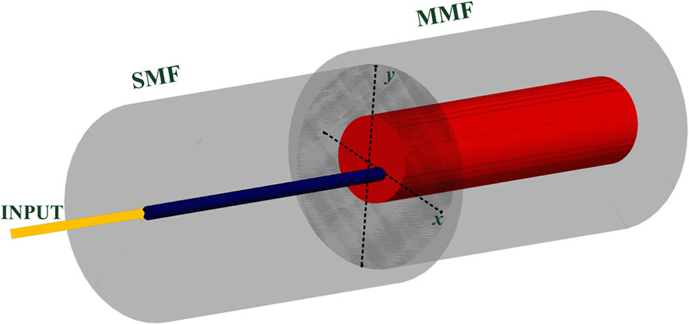
High-order modes tend to be excited in MMF if the SMF and MMF are offset spliced with each other^[25]. Figure 1 illustrates a schematic of the offset splicing of the two fibers. Assuming that no offset exists in the process of splicing, the union of the distal surface of the SMF and front surface of the MMF is centrosymmetric, but that turns to axisymmetric if the centers of the SMF and MMF do not coincide. From Ref. [8], we learn that the axisymmetric fundamental mode can be partly converted to the centrosymmetric higher-order mode at the offset splicing point. The proportion of each fiber mode under different offset splicing points is varied, and thus, we can derive different specklegrams in this way, which provides the potential to realize big data driven locations using the deep learning method.

When two different waveguides (such as an SMF and an MMF) are spliced together, the mode excitation ratio (MER) of the μth mode in the output waveguide can be expressed as ημ=[∬(E→in×H→μ*)·z^dxdy]2[∬(E→μ×H→μ*)·z^dxdy][∬(E→in×H→in*)·z^dxdy].(1)Here, E→in and H→in are the electromagnetic field distributions in the input waveguide, and the electromagnetic field distributions of the μth mode in output waveguide are represented by E→μ and H→μ. Once a coordinate system is defined, we can calculate the MER of each mode under different offset points. As shown in Fig. 1, the original point is set as the center of the MMF. The MMF we use in this Letter is the same as that in Ref. [8], which can support 110 vector modes, with a core diameter of 50 μm and the NA of 0.2. The SMF is SMF-28, and input light in the SMF is the y-polarized fundamental mode. We solve the electromagnetic field distribution of each mode using the finite element method.

Figure 2 illustrates the MERs of different modes in the MMF under different offset points in the x direction (the offset distance in the y direction is zero) at the wavelength of 1550 nm. Here, the order of the mode is arranged as the effective refractive index descends. Obviously, higher-order modes are easily excited in large offset distance situations, and the MER over the x axis is symmetric about the original point. Speckle intensity distribution is calculated by I(x,y)=|∑ν=1110ημE→μ(x,y)e−jβμz∬(E→in×H→in*)·z^dxdy|2.(2)Here, βμ is the propagating constant of the μth mode, and z represents fiber length. In the following analysis, the fiber length is fixed at 10 cm.

In the inset of Fig. 3, we perform the speckle patterns of five different offset points on the x axis. The mode speckle changes drastically and tends to centralize when the offset point varies from −25μm to 0 and discretizes as it goes up from 0 to 25 μm. To investigate the trend intuitively, an auto-correlation function of these specklegrams is defined in Eq. (3): Ψ(d)=∬i0iddxdy(∬i02dxdy∬id2dxdy)1/2,(3)where i represents the intensity distribution after removing the background light, i0 is the intensity distribution when there is no offset, and id is the intensity distribution over different offset points. Figure 3(a) depicts the auto-correlation function versus offset point in the x direction. Figure 3(b) is the auto-correlation function in the whole investigated plane, and the correlation value varies significantly in the whole plane, which is the basis of image feature recognition.

The aforementioned analysis points out how the offset point of the two fibers influences the MER. Figure 4 performs the excitation ratio of the particular modes over different offset points in the whole investigation plane. Coincidentally, the excitation efficiency distribution of the third and the seventh lower modes is centrosymmetric about the original point (the center of MMF), which is very similar to the linearly polarized LP11 mode and LP21 mode, respectively. Actually, Eq. (1) represents the vector overlap extent of two different modes. In our situation, the input fundamental mode in the SMF and modes in the MMF are centrosymmetric, and the MER profile of one specific mode in the MMF is dependent on its intensity profile in one polarization direction. Thus, we only need to study the situation of the half-plane to avoid identical speckle pattern, since the MER profile of every mode in the MMF is centrosymmetric. To testify to this, Figs. 5(a) and 5(b) show speckle distributions under two centrosymmetric offset points [(6μm, −5μm) and (−6μm, 5μm)], and they are identical. Meanwhile, as Fig. 3(b) shows, the correlation function in the whole plane is also centrosymmetric. That is to say, if we take the whole plane into consideration, identical specklegrams will be derived, and the prediction rate will decrease. In order to reduce wrong predictions, we only account for the points in the upper half-plane in Fig. 3(b).

Figure 6(a) shows the steps of data generating and processing. Firstly, MER is calculated using Eq. (1). Here, the interval in the x and y directions is 0.5 μm. In order to acquire more training data, the calculated MERs at different offset points are interpolated, and the amount of data quadruples that before interpolation. Thus, the total number of training and test data reaches 20,201. Secondly, specklegrams are constructed according to Eq. (2) using MERs obtained in the first step. The array size is limited to 102×102×1. Thirdly, the training and test data are converted to 8 bits images. The conversion equation is Ic(x,y)=I(x,y)−min[I(x,y)]max[I(x,y)]−min[I(x,y)],(4)where I(x,y) is the speckle intensity distribution. Also, all of the coordinates are normalized in the range of [0, 1] [the normalized coordinate is represented by (X, Y)]. The specklegrams are sent to trained CNN architecture in the fourth step, which is the most crucial step in the whole data processing system. As shown in Fig. 6(b), the CNN architecture contains four convolutional layers, four max pooling layers, and four fully connected layers. The size of each convolutional layer is 3×3 with strides of 1×1, and the number of filters is 16, 32, 64, and 128, successively. The activation function of each convolutional layer is a rectified linear unit (ReLU). After each convolutional layer, we set a max pooling layer with the size 2×2 and stride 1×1. Before being sent to the fully connected layer, the data is flattened to one dimension. The first three fully connected layers are 256 in size and use ReLU as the activation function. The last fully connected layer contains two neurons, which represents the predicted offset point, and the activation function is sigmoid. We randomly select a dataset containing 2000 specklegrams as the validation set, and another 18,201 specklegrams are assigned to the training set. The learning rate is set to 0.001, and the number of epochs is 30. In every epoch, mini batches with the size of 16 are sent to the CNN architecture.

Figure 7 shows the loss value under different epochs, which is defined by the mean square error (MSE) between the predicted and the labeled offset coordinates: MSE=1m∑i=1m[(Xp(i)−Xl(i))2+(Yp(i)−Yl(i))2].(5)Here, m is the number of validation samples. Normalized predicted and labeled offset coordinates are denoted by (Xp,Yp) and (Xl,Yl), respectively. After training for 30 epochs, the training loss ends up with 1.28×10−3, and the validation loss value is 1.31×10−3. The training results verify that our model begins to converge after training for two epochs, and no over-fitting or under-fitting exists.

To evaluate the effectiveness of our system, the relationship between the predicted and the labeled offset points is investigated. The distance difference between the predicted and labeled offset points is defined by d=(xp−xl)2+(yp−yl)2,(6)where (xp,yp) and (xl,yl) are actual coordinates rather than normalized coordinates of the predicted and labeled offset points. Figure 8 illustrates the distribution of distance difference. When d is less than 2 μm, the percentage reaches 98.55%. When d is within the range of 0 to 1.5 μm, the ratio is higher than 94%, which turns to 75.05% if d is less than 1 μm. The predicted result is reliable in micron horizon positioning. As Fig. 3(b) shows, the auto-correlation values are very close to each other in the range of 2 μm.

Figure 9 performs the labeled offset points with corresponding d higher than 2 μm. Nearly all of the points with larger error come from the line y=0 (x axis in the Cartesian coordinate system), especially in the situation where d is higher than 3 μm. As Fig. 3(a) shows, specklegrams on the x axis are centrosymmetric. Thus, when an offset point comes from this plane, except the line y=0, we can predict the offset coordinate accurately via the proposed CNN architecture.

In the future, we will try to verify our theoretical analysis in experiment. Since multimode speckle is sensitive to any perturbation in its surrounding environment, MMF should be short enough (not larger than 10 cm) and should hold in a customized fiber fixture. Besides, a high-precision translation platform is needed to adjust the offset point on the input plane of the MMF. The input SMF should be fixed to prevent twist-induced polarization variation.

In this Letter, we try to use a fixed position in the micron scale using CNN architecture. To the best of our knowledge, it is the first time that a fiber-based sensor is theoretically used to realize two-dimensional micro displacement sensing. Different offset points decide different specklegrams, which provides learning data to CNN architecture. Simulation results demonstrate that 98.55% predicted offset coordinates are within 2 μm of their corresponding labeled offset coordinates, and the rest of the predicted offset coordinates with large deviation mainly come from the border of the calculated domain. In all, the proposed method is effective for predicting offset coordinate between the SMF and MMF via specklegrams at the distal end of the MMF. We believe this work provides a very useful method for two-dimensional displacement measurement.