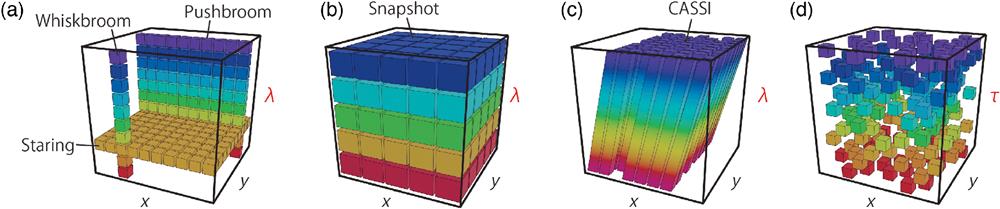
Fig. 1. Data acquisition of a 3D data cube in HSI. (a) Various scanning methods to obtain a 3D data cube in HSI. The pixels measured during a detector integration period are depicted for each scanning method. (b) Snapshot spectral imaging. (c) CASSI. (d) Data acquisition of CS-powered HSI. The data points in the 3D data cube are partially sampled and then processed to reconstruct the complete data set.

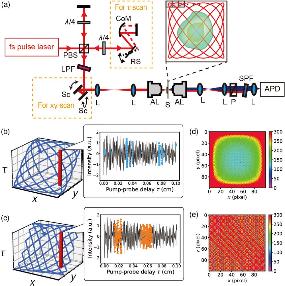
Fig. 2. CS-based FT-CARS imaging. (a) Schematic of the simulated experimental setup. AL, achromatic lens; APD, avalanche photodiode; CoM, concave mirror; L, lens; LPF, long-pass filter; P, polarizer; PBS, polarizing beam splitter; RS, resonant scanner; S, sample; Sc, scanner; SPF, short-pass filter; and λ/4, quarter-wave plate. (b), (c) Conceptual illustration of sinusoidal (b) and triangular (c) Lissajous scanning trajectories in 3D space spanned by positions (x,y) and optical delay τ. Typical sampling patterns at one spatial point are shown in the caption bubbles. (d), (e) Distributions of the number of sampled points with sinusoidal scanning (d) and triangular scanning (e) forxy scanning. The upper bound is set at 300 for both images.

Fig. 3. Selection of the hyperparameter values. RMSE values as a function of λ are shown. The measurement duration is 40 ms. Dashed lines represent the optimal values of λ.

Fig. 4. Numerical simulation of recovering undersampled data. (a) Assumed spectrum of a chemical and its concentration map. (b) Typical spectrum and intensity map at 1000cm−1 of sparsely sampled data obtained by pixel-wise NDFT without CS. (c), (d) Typical spectra and intensity maps at 1000cm−1 of the hyperspectral images reconstructed via CS from time-domain signals coarsely sampled with (c) sinusoidal Lissajous scanning (d) and triangular Lissajous scanning. The arrows in (b)–(d) indicate the points whose spectra are displayed.

Fig. 5. Performance of CS-powered time-domain HSI with different scanning functions. (a) Performance of CS-powered time-domain HSI with different compression ratios. The top axis represents the measurement time normalized by Traster, the measurement time in the raster-scan method. (b), (c) Intensity maps at 1000cm−1 and typical spectra with measurement durations of 30 ms with sinusoidal Lissajous scanning and triangular Lissajous scanning, respectively. (d) Performance of CS-powered time-domain HSI with different values of noise amplitudes and a measurement duration of 40 ms. (e), (f) Typical intensity maps at 1000cm−1 and typical spectra with a noise amplitude of 0.5 with sinusoidal Lissajous scanning and triangular Lissajous scanning, respectively. Arrows in (b), (c), (e), and (f) indicate the points whose spectra are displayed.

Fig. 6. Recovery of a spectral image of an E. gracilis cell by CS. (a), (c), (e) Intensity maps at 1000, 1300, and 1440cm−1 of hyperspectral images reconstructed via CS, respectively. (b), (d), (f) Intensity maps at 1000, 1300, and 1440cm−1 of hyperspectral images obtained by Fourier transform of generated time-domain interferograms, respectively. (g), (i) CS-reconstructed spectra at the points indicated by arrows in (a) and (c), respectively. (h), (j) Fourier transform of the generated time-domain interferograms at the points indicated by arrows in (b) and (d), respectively. (k) Performance of CS-based time-domain HSI for different measurement durations.