
Jianfeng Chen, Zhi-Yuan Li. Configurable topological beam splitting via antichiral gyromagnetic photonic crystal[J]. Opto-Electronic Science, 2022, 1(5): 220001
- Opto-Electronic Science
- Vol. 1, Issue 5, 220001 (2022)
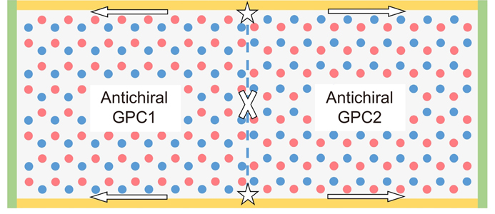
Fig. 1. Schematic illustration of antichiral gyromagnetic photonic crystal. GPC1 and GPC2 are oppositely magnetized, and their interface is marked by a blue dotted line. The white stars and arrows are the sources and the transport directions of edge states, and white cross indicates that the waveguide does not support any transmission. Only TE polarization (where electric field is parallel to z direction) is considered.
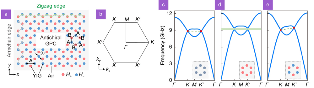
Fig. 2. Construction of antichiral gyromagnetic photonic crystal. (a ) Schematic illustration of antichiral GPC. The antichiral GPC possesses the zigzag and armchair edges along the x and y directions respectively. (b ) First Brillouin zone of honeycomb lattice. (c ) Nonmagnetized GPC. The nonmagnetic gyromagnetic cylinders are marked as the gray circles. The frequencies of Dirac points at K and K' points are 8.85 GHz. (d ) Uniformly magnetized GPC. All gyromagnetic cylinders are applied with external magnetic fields along +z (red) directions. The green region is the complete bandgap ranging from 9.10 to 9.40 GHz. (e ) Compound magnetized GPC. Two sublattices A and B are applied with external magnetic fields along –z (blue) and +z (red) directions respectively. The frequency of Dirac points (red points) at K and K' points is 9.10 GHz and 9.40 GHz respectively.
Fig. 3. Single antichiral gyromagnetic photonic crystal possessing zigzag and armchair edges. (a ) Experimental setup. (b ) Projected band structure along zigzag edge. (c ) Eigenmodal field profiles in panel (b). (d ) Calculated electric field distribution. (e ) Unprocessed transmission data at zigzag edge in simulation. (f –g ) Unprocessed transmission data measured at upper and lower zigzag edges respectively in experiment.
Fig. 4. Band structure and transport behavior along armchair edge. (a ) Projected band structure. (b ) Eigenmodal field profiles in (a). (c ) Electric field distribution of edge states propagating along zigzag-armchair waveguide. (d ) Electric field distribution of edge states propagating along armchair waveguide. In simulations, the green and yellow boundaries are set as scattering boundary conditions and perfect electric conductors respectively. The excitation frequency is 9.30 GHz. (e ) Unprocessed transmission data calculated at the right armchair edge in simulation. (f ) Unprocessed transmission data measured at the right armchair edge in experiment.
Fig. 5. Compound antichiral GPC supporting bidirectionally radiating one-way edge states. (a ) A clear look at the fabricated sample with the first and second layers removed. (b –c ) Simulation results of without and with metallic obstacles (yellow cylinders) respectively. The excitation frequency is 9.30 GHz. Unprocessed transmission data measured at four one-way waveguide channels (d –g ) without and (h –k ) with metallic obstacles.
Fig. 6. Variable-ratio topological beam splitting. (a –c ) Electric field distributions in simulation. The excitation frequency is 9.30 GHz. (d –f ) Unprocessed transmission data measured of S31 and S21 parameters. (g ) Normalized transmission data of S31 and S21 parameters in (d-f).


Set citation alerts for the article
Please enter your email address

© Copyright 2018-2021 | Chinese Laser Press. All Rights Reserved 沪ICP备15018463号-20