
Fengxun Gong, Mengran Li. Performance Analysis of Arrival Time Estimation Algorithm for Multilateration System[J]. Laser & Optoelectronics Progress, 2022, 59(13): 1304002
- Laser & Optoelectronics Progress
- Vol. 59, Issue 13, 1304002 (2022)
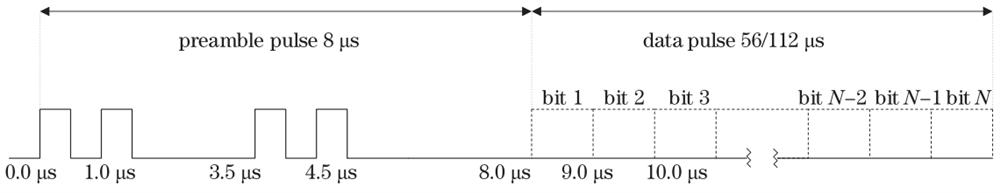
Fig. 1. Pulse string of the S-mode signal
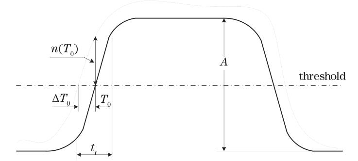
Fig. 2. Schematic diagram of TOA measured by rising edge decision algorithm
Fig. 3. Simulation results of the matched filtering algorithm
Fig. 4. Simulation results of the differential matched filtering algorithm
Fig. 5. Processing result of the differential matched filter to the multi-pulse. (a) M=2; (b) M=4
Fig. 6. TOA theoretical accuracy of different algorithms
Fig. 7. Fitting results of the RE algorithm
Fig. 8. Variation curve of the fitting effect of different order polynomial of DAE algorithm with SNR
Fig. 9. Influence of fitting order and data volume of DAE algorithm on fitting results. (a) Polynomial order; (b) data volume
Fig. 10. Fifth-order polynomial fitting result of the DAE algorithm
Fig. 11. Influence of SNR,
Fig. 12. TOA error distribution for different algorithms. (a) ME algorithm; (b) DE algorithm
Fig. 13. TOA estimation error distribution of DAE and ME algorithms. (a) SNR is 10 dB; (b) SNR is 15 dB
Fig. 14. Actual data acquired by the MLAT receiver. (a) Full data; (b) intercepted complete S-mode signal
Fig. 15. Actual arrangement of MLAT stations at international airports
Fig. 16. Root mean square error of TOA estimates for different algorithms
Fig. 17. Influence of different algorithms on the HDOP distribution of the MLAT system. (a) RE; (b) RAE; (c) ME; (d) DE; (e) DAE
Fig. 18. Influence of different algorithms on the VDOP distribution of the MLAT system. (a) RE; (b) RAE; (c) ME; (d) DE; (e) DAE
|
Table 1. Root mean square error extreme value and mean value of different algorithms

Set citation alerts for the article
Please enter your email address
© Copyright 2018-2021 | Chinese Laser Press. All Rights Reserved 沪ICP备15018463号-20