• Photonics Research
  • Vol. 9, Issue 5, B220 (2021)
Shanshan Zheng1、2, Hao Wang1、2, Shi Dong1、2, Fei Wang1、2, and Guohai Situ1、2、3、4、*
Author Affiliations
  • 1Shanghai Institute of Optics and Fine Mechanics, Chinese Academy of Sciences, Shanghai 201800, China
  • 2Center of Materials Science and Optoelectronics Engineering, University of Chinese Academy of Sciences, Beijing 100049, China
  • 3Hangzhou Institute for Advanced Study, University of Chinese Academy of Sciences, Hangzhou 310024, China
  • 4CAS Center for Excellence in Ultra-intense Laser Science, Shanghai 201800, China
  • show less
    DOI: 10.1364/PRJ.416246 Cite this Article Set citation alerts
    Shanshan Zheng, Hao Wang, Shi Dong, Fei Wang, Guohai Situ. Incoherent imaging through highly nonstatic and optically thick turbid media based on neural network[J]. Photonics Research, 2021, 9(5): B220 Copy Citation Text show less
    Incoherent scattering imaging experimental system. (1) and (2) are the captured scattered patterns (the raw data and corresponding partial contrast stretched map) with optical thickness of 8 and 16, respectively. Note that these data are recorded in two sets of experiments: (1) capture data by the camera directly; (2) capture data with two additional apertures placed before the camera. KLS, Köhler lighting system; P, polarizer; ambient light, generated by a high-power LED through a diffuse slate (the distance between the slate and the tank side was around 3.5 cm); camera, working with an imaging lens (f=250 mm, not shown in the figure). d1≃41 cm, d2≃15 cm. The 33.6 cm thick tank is equipped with fat emulsion diluent to simulate a dynamic scattering medium. Note that the scattered patterns shown in (2) look dimmed because a significant part of the large-angle scattered light has been blocked out.
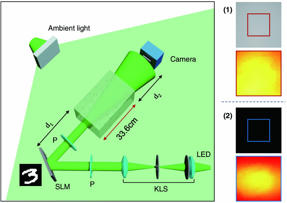
    Fig. 1. Incoherent scattering imaging experimental system. (1) and (2) are the captured scattered patterns (the raw data and corresponding partial contrast stretched map) with optical thickness of 8 and 16, respectively. Note that these data are recorded in two sets of experiments: (1) capture data by the camera directly; (2) capture data with two additional apertures placed before the camera. KLS, Köhler lighting system; P, polarizer; ambient light, generated by a high-power LED through a diffuse slate (the distance between the slate and the tank side was around 3.5 cm); camera, working with an imaging lens (f=250  mm, not shown in the figure). d141  cm, d215  cm. The 33.6 cm thick tank is equipped with fat emulsion diluent to simulate a dynamic scattering medium. Note that the scattered patterns shown in (2) look dimmed because a significant part of the large-angle scattered light has been blocked out.
    Optical thickness of intralipid suspensions with respect to its density. (b)–(j) Speckle patterns corresponding to different densities. Scale bar: 200 μm.
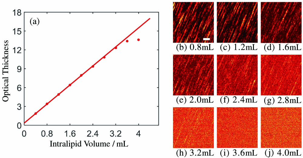
    Fig. 2. Optical thickness of intralipid suspensions with respect to its density. (b)–(j) Speckle patterns corresponding to different densities. Scale bar: 200 μm.
    Multiple scattering trajectories in dynamic media. In this illustration, scatterers move from the black circle to the blue circle during time interval Δτ, and ri (i=1,…,n,…,N) represents the location where scattering event occurs.
    Fig. 3. Multiple scattering trajectories in dynamic media. In this illustration, scatterers move from the black circle to the blue circle during time interval Δτ, and ri(i=1,,n,,N) represents the location where scattering event occurs.
    Experiment setup. (a) Dual camera acquisition system. (b) Experimental site map of intralipid dilution: 11.47 L purified water (33.6 cm×19.5 cm×17.5 cm) and 2 mL intralipid 20%.
    Fig. 4. Experiment setup. (a) Dual camera acquisition system. (b) Experimental site map of intralipid dilution: 11.47 L purified water (33.6cm×19.5cm×17.5  cm) and 2 mL intralipid 20%.
    Decorrelation curves for different concentrations of intralipid dilutions. The data points and the error bars represent the mean value and the standard error of the correlation coefficient calculated from 10 image pairs. The solid lines in different colors are the fitting results, and the corresponding intralipid volume VI and optical thickness (OT) are shown in the legend. Here, the coefficient of determination (R-square) is used to describe the goodness of fit. Note that the horizontal axis is logarithmic scale.
    Fig. 5. Decorrelation curves for different concentrations of intralipid dilutions. The data points and the error bars represent the mean value and the standard error of the correlation coefficient calculated from 10 image pairs. The solid lines in different colors are the fitting results, and the corresponding intralipid volume VI and optical thickness (OT) are shown in the legend. Here, the coefficient of determination (R-square) is used to describe the goodness of fit. Note that the horizontal axis is logarithmic scale.
    Experimental results. (a) Ground truths, and the reconstructed images in the case that the optical thickness equals (b) 8 and (c) 16, respectively.
    Fig. 6. Experimental results. (a) Ground truths, and the reconstructed images in the case that the optical thickness equals (b) 8 and (c) 16, respectively.
    Robustness against the position change of the object/camera. Δd is the displacement of the object/camera (in pixel). The data points and the error bars represent the mean values and the standard deviations of the SSIM/RMSE of 10 reconstructed images (digits ‘0–9’).
    Fig. 7. Robustness against the position change of the object/camera. Δd is the displacement of the object/camera (in pixel). The data points and the error bars represent the mean values and the standard deviations of the SSIM/RMSE of 10 reconstructed images (digits ‘0–9’).
    Robustness against the scaling and rotation of the object/camera. β is the scaling factor of the image size, Δθ the rotation angle, and Cg the image contrast gradient. The data points and the error bars in (a)–(d) represent the mean values and the standard deviations of the SSIM/RMSE of 10 reconstructed images (digits ‘0–9’). (e) and (f) SSIM/RMSE of digit ‘5’ with respect to Δθ and Cg. (g) Visualized reconstructed digits.
    Fig. 8. Robustness against the scaling and rotation of the object/camera. β is the scaling factor of the image size, Δθ the rotation angle, and Cg the image contrast gradient. The data points and the error bars in (a)–(d) represent the mean values and the standard deviations of the SSIM/RMSE of 10 reconstructed images (digits ‘0–9’). (e) and (f) SSIM/RMSE of digit ‘5’ with respect to Δθ and Cg. (g) Visualized reconstructed digits.
    Reconstruction of nondigit objects with the neural network trained by using digits. (a) First and third rows are the ground truths; second and fourth are the corresponding reconstructed images. (b) Reconstructed USAF target and the highlight of some of its portions.
    Fig. 9. Reconstruction of nondigit objects with the neural network trained by using digits. (a) First and third rows are the ground truths; second and fourth are the corresponding reconstructed images. (b) Reconstructed USAF target and the highlight of some of its portions.
    Experimental results with natural scene object. (a) Scattered patterns. (b) Corresponding ground truth. (b) Reconstructed results.
    Fig. 10. Experimental results with natural scene object. (a) Scattered patterns. (b) Corresponding ground truth. (b) Reconstructed results.
    Proposed neural network architecture. (a) Digits in the format m−n below each layer denote the number of input channels m, and the number of output channels n. (5, 5) and (3, 3) denote the size of the convolution kernel in pixel counts. (b) Detailed information of neural network structure.
    Fig. 11. Proposed neural network architecture. (a) Digits in the format mn below each layer denote the number of input channels m, and the number of output channels n. (5, 5) and (3, 3) denote the size of the convolution kernel in pixel counts. (b) Detailed information of neural network structure.
    Shanshan Zheng, Hao Wang, Shi Dong, Fei Wang, Guohai Situ. Incoherent imaging through highly nonstatic and optically thick turbid media based on neural network[J]. Photonics Research, 2021, 9(5): B220
    Download Citation