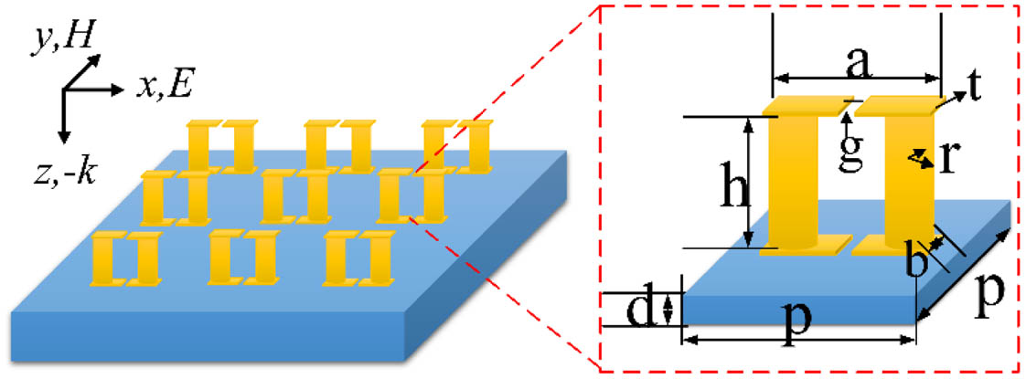
Fig. 1. 3D schematic drawing of the proposed metamaterial sensor and a single enlarged unit cell with its geometrical dimensions. The inset shows the polarization of the EM wave illumination. The electric field component is vertical to the gap of the DVSRRs. The magnetic field is normal to the DVSRR. The EM wave illuminates from the top perpendicularly. The geometric parameters of a single DVSRR unit cell are a=50  μm, b=12  μm, t=1  μm, h=30  μm, r=6  μm, and g=2  μm. The period of the square lattice is p=70  μm.

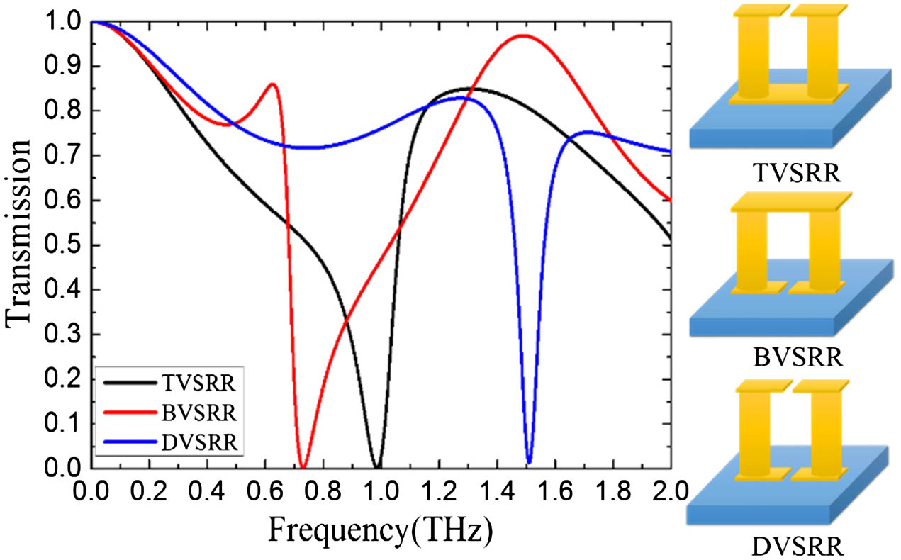
Fig. 2. Comparison of the transmission spectra of three different VSRRs that share the same dimensions, except for the positions and number of gaps. The TVSRR and BVSRR display the VSRRs with one slot in the top or bottom metal plate, respectively.

Fig. 3. Comparison of the numerically calculated distributions of the three VSRR structures at resonant frequencies, namely 0.9853, 0.7305, and 1.5102 THz for TVSRR, BVSRR, and DVSRR respectively. (a), (d), and (g) illustrate the surface current distributions for the three VSRRs. The black arrows denote the directions of surface electric current. (b), (e), and (h) show the magnetic energy density distributions. The electric energy density distributions are also shown in (c), (f), and (i). The electric energy density in the lower gap of the DVSRR is enlarged and demonstrated in the red dotted line box in the inset of (i).

Fig. 4. (a) 3D sketch diagram of the sensing configuration including the DVSRR’s array sensor and analyte. The sensing performance based on the thicknesses and RIs of the analyte are shown in the following subgraphs. (b) The transmission spectra of the DVSRR with and without analyte overlaid on the sensor. Analytes with the different thicknesses (l=2–7  μm) and constant n=1.6 are used in the numerical calculations of (b). To observe more clearly the sensing evolution, a break for the coordinate values in the horizontal axis has been introduced. (d) The fitting function using the data from (b) between the FS of the resonant dip and analyte thickness are shown. (c) Different transmission spectra are induced by the increasing RI (n=1–1.9) and constant l=6  μm of the analyte. (e) The exponential fitting curve for the data shown in (c) are displayed as the black curve, which can be expressed as FS=0.92464−2.326035*exp(−0.96198*n) with R2=0.99992. The RI sensitivity of the DVSRR is also displayed as the blue curve in (e).

Fig. 5. Comparative plots of (a) thickness sensing with fixed RI of n=1.6 and (b) RI sensing with constant thickness l=6  μm among the three structures: TVSRR, BVSRR, and DVSRR. A break is added in the y axis of (a) to manifest the values of FS for different VSRRs. (c) The bar plot shows the proportion of FS for n=1.1–2 induced by the analyte filling within the two gaps of DVSRR.

Fig. 6. (a) 3D schematic drawing of the transmission spectral comparison for various DVSRR structures with fabrication tolerance ranging from −4% to 4%. Fabrication toleration is supposedly induced by inaccuracy in the fabrication process, which is calculated as a common coefficient of all the structural dimensions of the DVSRR. The sign “±” represents enlarging or shrinking all the structural dimensions of the DVSRR. (b) The Q-factor of the resonance of the DVSRR is shown as a function of fabrication tolerance (blue curve). The black curve shows the FS of its resonance dip induced by the analyte with n=1.6 and thickness l=6  μm versus fabrication tolerance.

Fig. 7. Transmission spectral comparison for (a) TM and (b) TE incidence radiation with increasing incidence angles with a step of 10°. The polarizations of the two incidence radiations are shown as the insets in (a) and (b).

Fig. 8. 3D bar plots shows the evolution of the sensing performance of the DVSRR for a wide range of incidence angles (0°–50°) and the increasing RI (1.2–2) with fixed thickness l=6  μm under (a) TM and (b) TE incidence radiation. (c) The numerically calculated results of the FS induced by the analyte with n=1.6 and l=6  μm are shown as a function of the incidence angles for the TM and TE illumination, selected as examples to illustrate that the sensing performance of the DVSRR is incidence-angle-insensitive in the range of 0°–50°.