
Kun Huang. On the applicability of adiabatic approximation in multiphonon recombination theory[J]. Journal of Semiconductors, 2019, 40(9): 090102
- Journal of Semiconductors
- Vol. 40, Issue 9, 090102 (2019)
Abstract
By considering F-centers, we based on adiabatic approximation have proposed a theory for non-radiative transitions of electrons involving multi-phonon absorption or emission[
![]()
Figure 1.
We call it an “nonadiabatic” operator, as it reflects the fact that the lattice moves at a finite speed, thereby causing the transition to occur between the adiabatic wave functions (assuming that lattice motion is infinitely slow relative to electron motion).
Recently, C. V. Henry and D. V. Lang from Bell Labs in the United States published a very valuable paper based on their study on deep levels[
Similar to the model shown in Fig. 1, Henry and Lang mainly adopted a single coordinate model and calculated transition rates in the semiclassical approximation, where the lattice coordinate Q was considered as a parameter that changed with time. They assumed that the adiabatic wave functions ϕi(xQ) and ϕj(xQ) are existed only when the lattice has a distance from the intersection Qc in a range larger than |Q1 – Qc|. Then, the wave functions ϕi(xQ1) and ϕj(xQ1) at point Q1 were considered as the basis to describe these two states. The interaction in the vicinity of the intersection point beyong Q1 (i.e., |Q – Qc| < | Q1 – Qc|) was defined as the perturbation
where HeL(xQ) represents the interaction Hamiltonian of electrons with lattice motions. Regarding the breakdown of the adiabatic approximation near the intersection point C, they selected a specific value for Q1 (in fact they determined the energy difference between two electronic levels at Q1) as the applicable range for the adiabatic approximation. In this manner, they calculated the probability of a transition from φi(xQ1) to φj(xQ1) under ΔV perturbation whenever Q goes through the intersection Qc,
where
It is readily shown that if the adiabatic approximation near Qc indeed breaks down, and Q1 represents its limit of range, then the value of Q1 should have a clear physical meaning. With this in mind when we inspect the paper by Henry and Lang, we can see that the energy difference ε1 between two energy levels at Q1 given as 0.06 eV is obtained when the following parameter equals 1:
This formula leads to the following equation:
What physical meaning does this formula contain? The uncertainty principle offers a clue about this, where ε1 draws an area near the intersection Qc, and the time required to travel through this area can be written as:
This equation can be used to deduce the following uncertainty in energy:
It is shown that the law of the conservation of energy does not require the non-radiative transition occuring exactly at the intersection C where the two energy levels degenerate completely. A transition may occur as long as their energy difference is within the following range,
From Eq. (8) we could obtain the value of ε1.
which is basically consistent with the value as shown in Eq. (5) given by Henry and Lang.
Henry and Lang initially believed that the adiabatic approximation was no longer applicable within the range of the aforementioned energy difference, based on their observation that, within this range, the perturbation wave function began deviating from the wave function in adiabatic approximation. The deduction based on the aforementioned uncertainty principle indicates, however, that ε1 draws a region where a transition can occur near the intersection. From this point of view, it is natural that Henry and Lang found that the wave function deviated from the adiabatic wave function. This deviation simply reflects a fact that the transition induces the admixture of other states in the wave function. However, this deviation by no means announces the break down of the adiabatic wave function itself.
Therefore, the theory proposed by Henry and Lang (H–L theory) and the adiabatic approximation just represent two different approximation methods: H–L theory selects φi(xQ1) and φj(xQ1) as basis to approximate two states, and considers ΔV when Q falls near point C as a perturbation to calculate the transition probability between two states; the theory of adiabatic approximation is however, assuming that lattice Q changes very slowly, using the adiabatic wave functions Qi(xQ) and Qj(xQ) to describe approximately two electronic states and considering the non-adiabatic operator as the perturbation to calculate the transition probability. There is no reason to believe that these two practices are antagonistic and mutually exclusive.
In this case, the reasonable question is: which of the two approximation methods provides more accurate results? It is not difficult to compare the two methods via a direct calculation for simple linear electron-lattice interactions in a single-coordinate model,
According to the H–L theory,
the transition probability is obtained by inserting it into Eq. (3),
where the denominator is the rate of change of the energy difference
![]()
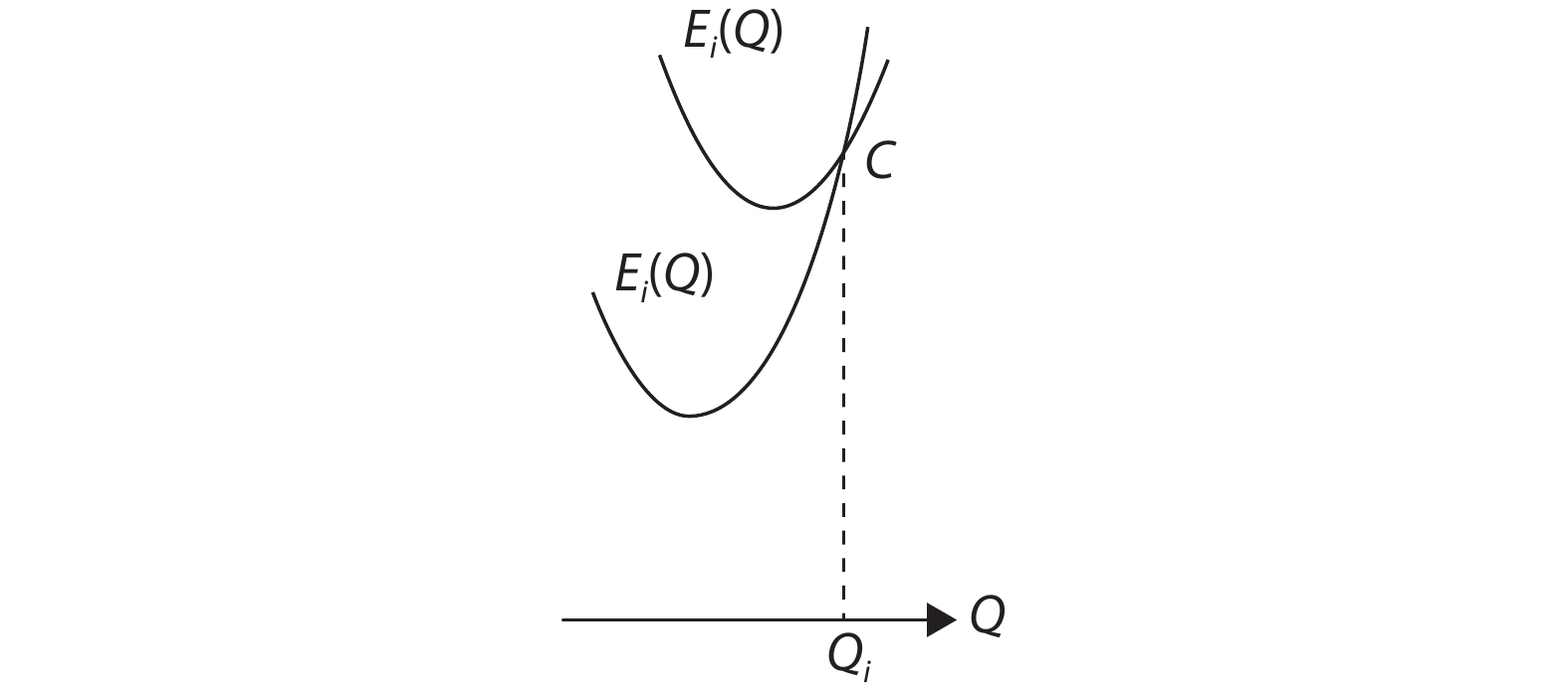
Figure 2.
On the other hand, the calculations according to the adiabatic approximation can be conducted relying directly on the formula given in the Landau-Lifschitz “quantum mechanics”[
where (F2 – F1) is defined as follows:
Although V is a non-adiabatic operator, it is expressed as a variable of classical mechanics. Employing the first-order perturbation theory, we choose φi(xQ1) and ϕj(xQ1) as the zero-order wave functions, and ΔV = u(x)(Q – Q1) as the perturbation to obtain the adiabatic wave functions and the eigen values Ei(Q) and Ej(Q), in a way as shown in Fig. 2. From this, Eq. (14) becomes:
Similarly, utilizing this type of first-order approximation adiabatic wave functions, we can obtain the non-adiabatic operator and further express it as a variable of classical mechanics:
Relying on Eq. (7) and Eq. (9), we can rewrite Eq. (16) as:
where Δt represents the time that Q travels from Q1 to Qc, and thus Eq. (17) becomes:
By inserting Eq. (15) and Eq. (18) into Eq. (13), we obtain the transition probability as
We can see that this result obtained from the adiabatic approximation is in complete agreement with Eq. (12) obtained from the H–L theory. Furthermore, two different approximation methods give rise to a completely consistent result, demonstrating the reliability of result.
Kubo and Toyozawa also pointed out another important problem on the transition occurring through energy intersections. As the degeneracy of the two energy levels at the intersection is often the only result of the first-order perturbation theory, any further considerations of the effect of the perturbation will lift such energy degeneracy and, therefore, give rise to separation between two energy levels as shown in Fig. 3. Consequently, the proper theory should calculate the transition probability based on the framework lifting this type of degeneracy. Plenty of theoretical work remain to be conducted in this area. One puzzle remains from the previous discussion: Why did we use previous theories without considering this issue but obtain results that are consistent with each other and seem reliable?
![]()
Figure 3.
To explain this problem, instead of using the aforementioned first-order adiabatic wave functions, we utilize a 2 x 2 Hamiltonian matrix in a basis of φi(xQ1) and φj(xQ1),
By diagonalizing the matrix, we can determine adiabatic wave functions in a higher precision. In this way, the degeneracy of the energy levels at the intersection is practically eliminated. Solving the secular equation corresponding to Eq. (20), we obtain the eigen values:
To obtain this equation, we have introduced the condition in which energy levels cross at Q = Qc in the first-order approximation:
We can now distinguish two scenarios under extreme conditions:
A. In Eq. (21), the second term is negligible in the comparison with the first term. It is straightforward to demonstrate that, in this case, the solution will return back to the results of the first-order approximation theory used previously. Obviously, it is the case at the boundary of the transition region (i.e., Q
B. In Eq. (21), the first term is negligible in the comparison with the second term (this is obviously the case at the intersection Q
is changing from
to
Therefore, the assumption of
renders most of the transition regions from Q1 to Qc are in accord with Case A, and subsequently the first-order approximation adiabatic theory adopted previously will be applicable and, accordingly, the H–L theory is valid. This is the case for transitions from a free state to a bound state or visa versa, such as the carrier capture process considered by the H–L theory, (because “
Acknowledgements
We would like to thank Prof. Jun-Wei Luo from the Institute of Semiconductors CAS for the translation of this article.
Special notes
(1) The article was originally published in Chinese in the first issue of Volume 1 of Chinese Journal of Semiconductors (K Huang. On the Applicability of Adiabatic Approximation in Multiphonon Recombination Theory. Chin J Semicond, 1980, 1(1), 1).
(2) Its republication in English version after 40 years is to commemorate Prof. Kun Huang's Centenary Birthday.
References
[1]
[2]
[3]
[4]


Set citation alerts for the article
Please enter your email address

© Copyright 2018-2021 | Chinese Laser Press. All Rights Reserved 沪ICP备15018463号-20