• Chinese Optics Letters
  • Vol. 20, Issue 11, 111901 (2022)
Jifang Rong1, Yiwu Ma1, Meng Xu2、**, and Hua Yang1、*
Author Affiliations
  • 1College of Computer Science and Electronic Engineering, Hunan University, Changsha 410082, China
  • 2School of Geosciences and Info-Physics, Central South University, Changsha 410083, China
  • show less
    DOI: 10.3788/COL202220.111901 Cite this Article Set citation alerts
    Jifang Rong, Yiwu Ma, Meng Xu, Hua Yang. Interactions of the second-order solitons with an external probe pulse in the optical event horizon[J]. Chinese Optics Letters, 2022, 20(11): 111901 Copy Citation Text show less
    (a) Wavenumber and corresponding group delay curve as a function of normalized angular frequency offset. The probe pulse is launched at a frequency offset such that the group velocities of the probe pulse and the soliton are equal. The temporal and spectral evolutions of the input field under the condition of GVM are shown in (b) and (c), respectively. (d) The corresponding spectrograms at different propagation lengths. In (b), (c), and (d), P0 = 1, AP = 0.1, δ = 25, t1 = 10, T1 = 3.
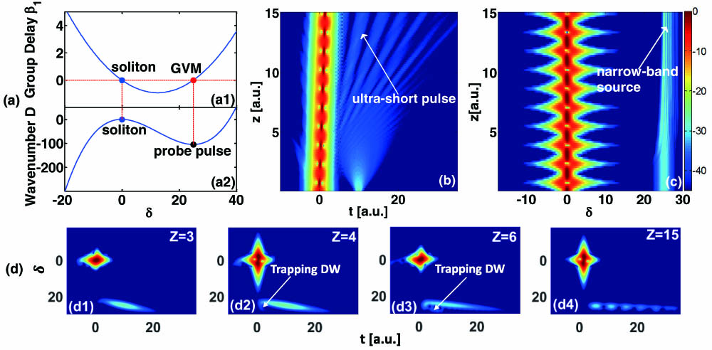
    Fig. 1. (a) Wavenumber and corresponding group delay curve as a function of normalized angular frequency offset. The probe pulse is launched at a frequency offset such that the group velocities of the probe pulse and the soliton are equal. The temporal and spectral evolutions of the input field under the condition of GVM are shown in (b) and (c), respectively. (d) The corresponding spectrograms at different propagation lengths. In (b), (c), and (d), P0 = 1, AP = 0.1, δ = 25, t1 = 10, T1 = 3.
    (a1) Spectral and (c2) temporal evolutions of the interaction between a probe pulse and a second-order soliton under the condition of GVMM. The corresponding wavenumber curve is shown in (a2). S and P represent the launch positions of the second-order soliton and the probe pulse, respectively. DW indicates the predicted position of the dispersive wave, G stands for the GVM point, and I denotes the position of the idle wave. (a3), (b1), and (b2) are zoomed-in plots of the spectrum in the green and red boxes in (a1). The output spectrum of the oscillating radiation region when adjusting the (d1) temporal width and (d2) time delay of the incident probe pulse based on (a1). (c1) The output temporal profile. In (b2), (d1), and (d2), the vertical dashed lines indicate the locations of the pairs of the probe and idle waves, which agree with Eq. (8) quite well (as indicated by the horizontal solid lines). Here, P0 = 1, AP = 0.1, δ = 22.62, T1 = 3.
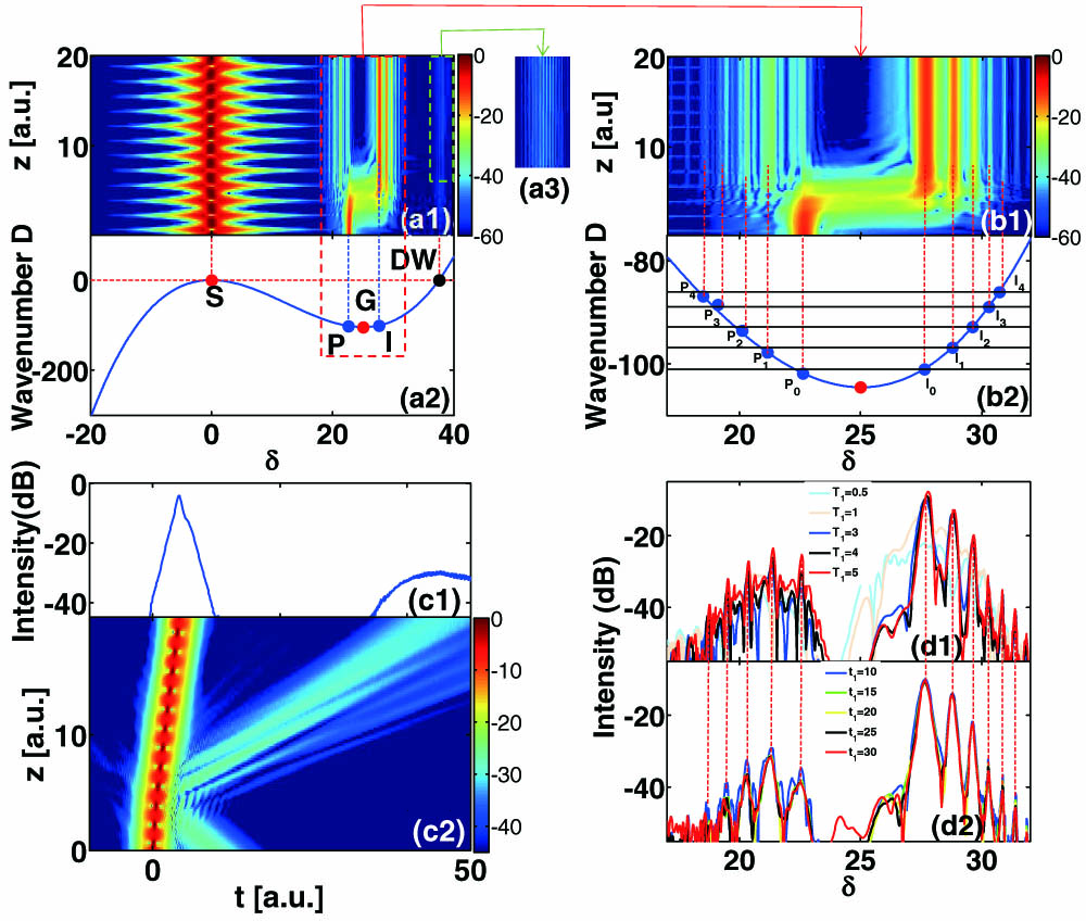
    Fig. 2. (a1) Spectral and (c2) temporal evolutions of the interaction between a probe pulse and a second-order soliton under the condition of GVMM. The corresponding wavenumber curve is shown in (a2). S and P represent the launch positions of the second-order soliton and the probe pulse, respectively. DW indicates the predicted position of the dispersive wave, G stands for the GVM point, and I denotes the position of the idle wave. (a3), (b1), and (b2) are zoomed-in plots of the spectrum in the green and red boxes in (a1). The output spectrum of the oscillating radiation region when adjusting the (d1) temporal width and (d2) time delay of the incident probe pulse based on (a1). (c1) The output temporal profile. In (b2), (d1), and (d2), the vertical dashed lines indicate the locations of the pairs of the probe and idle waves, which agree with Eq. (8) quite well (as indicated by the horizontal solid lines). Here, P0 = 1, AP = 0.1, δ = 22.62, T1 = 3.
    (a1)–(c1) The temporal and (a2)–(c2) spectral evolutions of the collision process between two well-separated second-order solitons and a probe pulse with different amplitudes AP: (a) 0.1, (b) 0.2, (c) 0.05. The white boxes are the partial enlargement of the corresponding white dotted boxes. Here, the other parameters of the simulation are the same as those used in Figs. 2(a1) and 2(c).
    Fig. 3. (a1)–(c1) The temporal and (a2)–(c2) spectral evolutions of the collision process between two well-separated second-order solitons and a probe pulse with different amplitudes AP: (a) 0.1, (b) 0.2, (c) 0.05. The white boxes are the partial enlargement of the corresponding white dotted boxes. Here, the other parameters of the simulation are the same as those used in Figs. 2(a1) and 2(c).
    Collision distance of the two main solitons, Zc, as a function of (a) the amplitude AP and (b) the temporal width T1 of the incident probe pulse. The width of the probe pulse is fixed at T1 = 3 in (a), while the amplitude of the probe pulse is fixed at AP = 0.1 in (b).
    Fig. 4. Collision distance of the two main solitons, Zc, as a function of (a) the amplitude AP and (b) the temporal width T1 of the incident probe pulse. The width of the probe pulse is fixed at T1 = 3 in (a), while the amplitude of the probe pulse is fixed at AP = 0.1 in (b).
    Jifang Rong, Yiwu Ma, Meng Xu, Hua Yang. Interactions of the second-order solitons with an external probe pulse in the optical event horizon[J]. Chinese Optics Letters, 2022, 20(11): 111901
    Download Citation