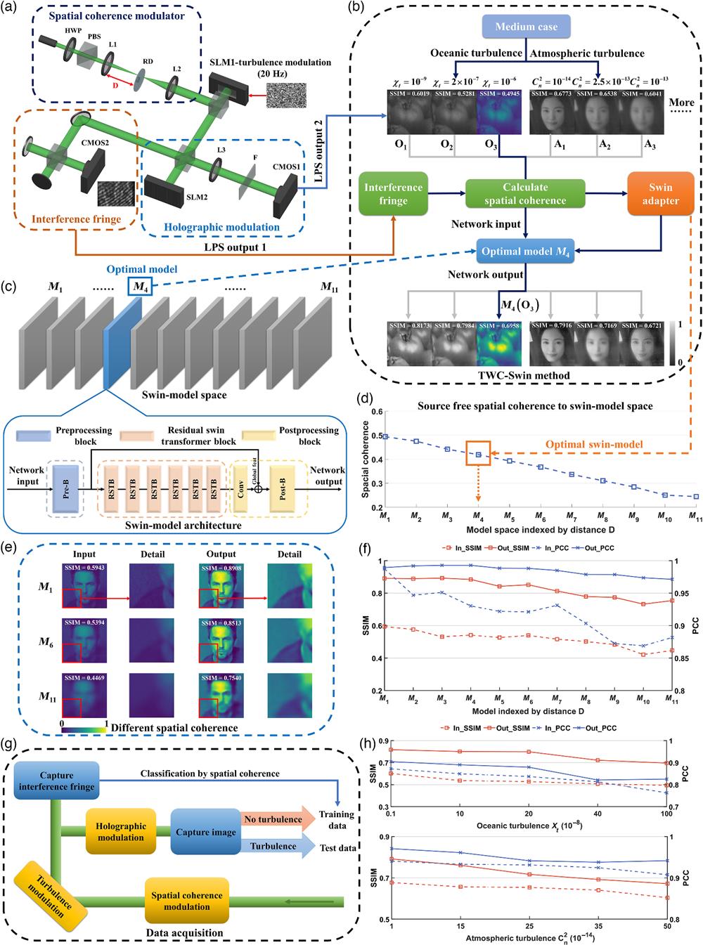
Fig. 1. Principle and performance of TWC-Swin method. (a) LPR. SC modulation can adjust the SC by changing the distance D. Holographic modulation is used to load the phase hologram. The LPR generates two outputs, one for calculating SC and the other for network input. HWP, half-wave plate; PBS, polarized beam splitter; L, lens; RD, rotating diffuser; SLM, spatial light modulator; F, filter. D, distance between L1 and RD. (b) The detailed flow of the TWC-Swin method. The swin adapter can select the optimal model from the model space by obtaining SC. The color picture represents a case in progress. (c) Swin-model space and architecture of the swin model. The architecture of M1−M11 is the same; only the weights are different. The weights are obtained by network training at different distances. (d) The correspondence between SC and swin-model space. See Table S1 in the Supplementary Material for detailed data. (e) Inputs and outputs of the swin model with different SCs. (f) SSIM and PCC of swin-model outputs at different SCs. (g) Training and test data acquisition process. The training data did not contain any turbulence. (h) SSIM and PCC of swin-model outputs at different turbulent scenes.

Fig. 2. Qualitative analysis of our method’s performance at the different SCs. Input, raw image captured by CMOS1. Output, image processed by the network. (a)–(k) Different SCs: (a) D=f1, SC is 0.494; (b) D=1.1f1, SC is 0.475; (c) D=1.2f1, SC is 0.442; (d) D=1.3f1, SC is 0.419; (e) D=1.4f1, SC is 0.393; (f) D=1.5f1, SC is 0.368; (g) D=1.6f1, SC is 0.337; (h) D=1.7f1, SC is 0.311; (i) D=1.8f1, SC is 0.285; (j) D=1.9f1, SC is 0.25; and (k) D=2f1, SC is 0.245. D means the distance between L1 and RD in the LPR and f1 is the focal length of L1. Our method can achieve improved image quality under low SC (Video 1, MP4, 1.5 MB [URL: https://doi.org/10.1117/1.AP.5.6.066003.s1]).

Fig. 3. Average results of the evaluation indices for each test data set. The coherence is 0.368. Results of other coherences are provided in Fig. S2 in the Supplementary Material. All evaluation indices demonstrate that our method possesses strong image restoration ability under low SC.

Fig. 4. Qualitative analysis of our method’s performance across varying intensities of (a) oceanic and (b) atmospheric turbulence. The network trained with coherence as physical prior information can effectively overcome the impact of turbulence on imaging and improve image quality. (O1)–(O5) mean oceanic turbulence phase and (A1)–(A5) mean atmospheric turbulence phase. (O1) χt=10−9K2/s, coherence is 0.491. (O2) χt=10−7K2/s, coherence is 0.482. (O3) χt=2×10−7K2/s, coherence is 0.447. (O4) χt=4×10−7K2/s, coherence is 0.404. (O5) χt=10−6K2/s, coherence is 0.373. (A1) Cn2=10−14m3−α, coherence is 0.507. (A2) Cn2=1.5×10−13m3−α, coherence is 0.459. (A3) Cn2=2.5×10−13m3−α, coherence is 0.43. (A4) Cn2=3.5×10−13m3−α, coherence is 0.403. (A5) Cn2=5×10−13m3−α, coherence is 0.378. Other parameter settings of the turbulent power spectrum function can be found in Table S2 in the Supplementary Material (Video 2, MP4, 36.4 MB [URL: https://doi.org/10.1117/1.AP.5.6.066003.s2]).

Fig. 5. Visualization of performance of different methods. The SSIM is shown in the bottom left corner. Our method presents the best performance, which is shown by smoother images with lower noise. (a) Sample selected with the WED data set and magnified insets of the red bounding region. (b) Sample selected with Flickr data set and magnified insets of the red bounding region. The pure swin model can be obtained by removing the postprocessing block of the swin model (Video 3, MP4, 0.6 MB [URL: https://doi.org/10.1117/1.AP.5.6.066003.s3]).

Fig. 6. Performance between different methods on various data sets with SC being 0.494. Our model outperforms other methods across various data sets and indices.

Fig. 7. (a), (b) Performance comparison between different methods at various turbulent scenes. (A1) Cn2=10−14m3−α, coherence is 0.506. (A2) Cn2=1.5×10−13m3−α, coherence is 0.459. (O1) χt=10−9K2/s, coherence is 0.491. (O2) χt=10−7K2/s, coherence is 0.482. Note that all methods are trained with coherence as physical prior information and improve image quality under turbulence conditions. This demonstrates that incorporating appropriate physical prior information can help the network cope with multiscene tasks.

Table 1. Quantitative analysis of evaluation indices (SSIM and PCC) at different SCs and test samples^a. f1 is the focal length of L1. SC means spatial coherence of the light source.

Table 2. Quantitative analysis of evaluation indices (SSIM and PCC) at different oceanic turbulence intensities^a.

Table 3. Quantitative analysis of evaluation indices (SSIM and PCC) at different atmospheric turbulence intensities^a.