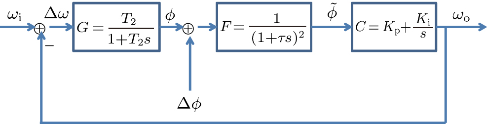
Fig. 1. The block diagram of the close-loop control of a quantum sensor system. The open-loop transfer function of the oscillator is denoted by G. A second order filter F with filter time constant τ is applied to suppress high frequency noise. A PI-controller C is used to adjust the output frequency ω_o so as to trace the variation of the input frequency ω_i. The control parameter K_p represents the proportional term and K_i stands for the integral term. The quantum phase white noise Δϕ will be a disturbance to the output of the PI-controller. Finally, the phase shift ϕ is the output of the sensor, followed by the high-frequency-noise-filtered phase shift ϕ∼.

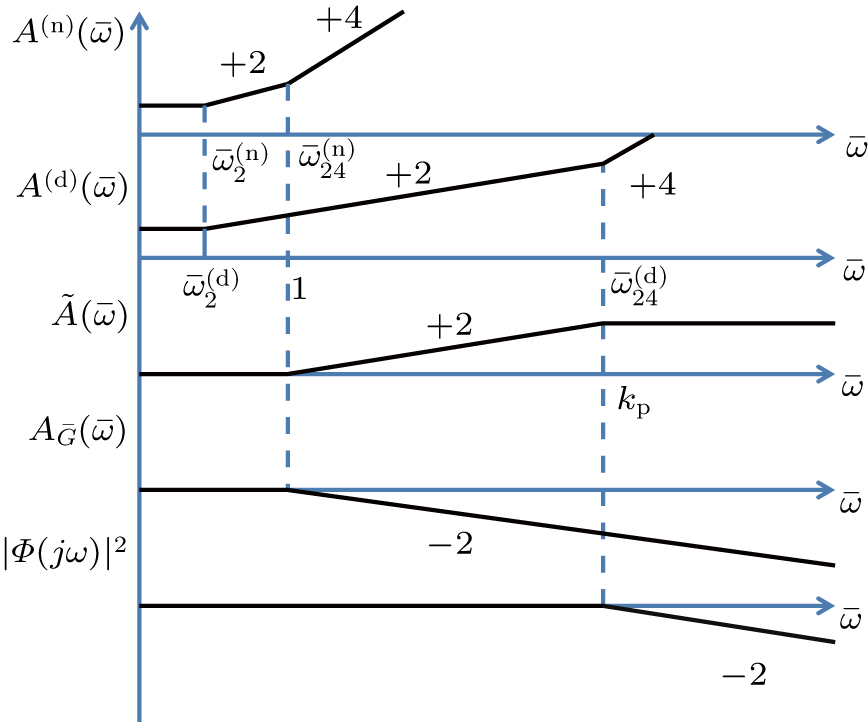
Fig. 2. Schematic diagram of bandwidth improvement by PID feedback. These curves are depicted in the log–log coordinates, where A(n)(ω¯) and A(d)(ω¯) represent the numerator and denominator of A∼(ω¯), respectively. The numbers +2 and +4 indicate that the terms proportional to ω¯2 and ω¯4 are dominant in those frequency intervals. The number –2 indicates that the functions decay as 1/ω¯2 in those frequency intervals.

Fig. 3. Demonstrations of the resonant and non-resonant behaviors of the close-loop frequency responses A_close(ω). The black curve represent the regime k_i ≪ k_p, while the red curve present resonant behavior with ki>kic. In this graph, k_p = 100 and k_i = (1 + k_p)².

Fig. 4. Comparisons of frequency responses with filter F present or not. The black curve represents the frequency response of the open-loop system G. The pink and green curves describe the close-loop frequency responses of Φ₁(s) = CGF/(1 + CGF) and Φ₂(s) = CG/(1 + CG) when the filter F is present or not, respectively. The blue and red curves correspond to the frequency responses of A₁(s) = CF/(1 + CGF) and A₂(s) = A(s), respectively. The parameters used in this graph are T₂ = 10 s, τ = 10⁻⁴ s, k_p = 1000 and k_i = 100.

Fig. 5. (a) The block diagram of the noise transfer. The noise Δϕ(s), which is here the Laplace transformation of Δϕ(t), causes a output frequency fluctuation in the PI controller, as represented by ω_n(s) in the above diagram. (b) The power spectral density Sn1/2(ω) of the noise output ω_n(t). The red curve is depicted with k_p = 2000, which is twice over that of the black one. Other parameters used are k_i = 100, T₂ = 10 s, τ/T₂ = 10⁻⁵, and T₂g = 10³.