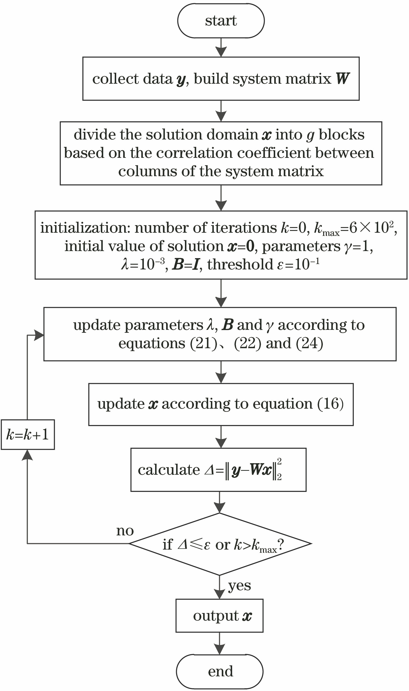
Fig. 1. Flow chart of proposed algorithm

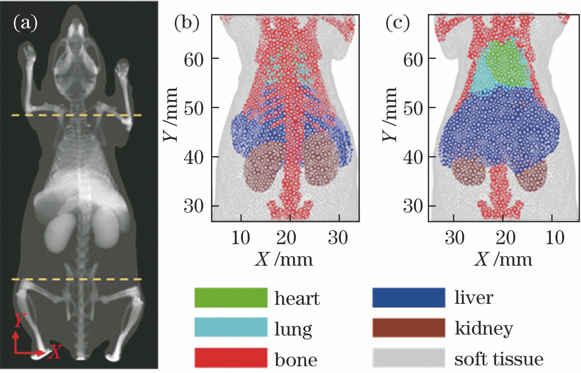
Fig. 2. Simulation models. (a) Heterogeneous digi-mouse model; (b) front view of discretized mesh of mouse torso; (c) back view of the discretized mesh

Fig. 3. Reconstruction results of single source in liver (all BLT results are normalized intensity). (a) 3D rendering of true source distribution; (b1)-(b3) transverse, coronal and sagittal views of true source overlapped with CT images; (c) 3D rendering of BSBL reconstruction result; (d1)-(d3) transverse, coronal and sagittal views of BSBL reconstruction result overlapped with CT images; (e) 3D rendering of L1-LS reconstruction result; (f1)-(f3) transverse, coronal and sagittal views of L1-LS reconstru

Fig. 4. Comparison of evaluation parameters of simulated results. (a) Comparison of 3D COM offset of reconstructed resource; (b) comparison of Dice coefficient between reconstructed and true sources; (c) comparison of αCNR of reconstructed image

Fig. 5. Reconstruction results of single source in kidney (all BLT results are normalized intensity). (a) 3D rendering of true source distribution; (b1)-(b3) transverse, coronal and sagittal views of true source overlapped with CT images; (c) 3D rendering of BSBL reconstruction result; (d1)-(d3) three views of BSBL reconstruction result overlapped with CT images; (e) 3D rendering of L1-LS reconstruction result; (f1)-(f3) three views of L1-LS reconstruction result overlapped with CT images

Fig. 6. Reconstruction results of single source in abdomen (all BLT results are normalized intensity). (a) 3D rendering of true source distribution; (b1)-(b3) transverse, coronal and sagittal views of true source overlapped with CT images; (c) 3D rendering of BSBL reconstruction result; (d1)-(d3) three views of BSBL reconstruction result overlapped with CT images; (e) 3D rendering of L1-LS reconstruction result; (f1)-(f3) three views of L1-LS reconstruction result overlapped with CT images

Fig. 7. Reconstruction results of double sources in lungs (all BLT results are normalized intensity). (a) 3D rendering of true source distribution; (b1) (b2) transverse and coronal views of true left source overlapped with CT images; (b3)(b4) transverse and coronal views of true right source; (c) 3D rendering of BSBL reconstruction result; (d1)(d2) transverse and coronal views of left source overlapped with CT images using BSBL method; (d3)(d4) transverse and coronal views of right source using BSBL met

Fig. 8. Normalized source intensity on line AB. (a) Schematic of line AB across single source; (b) schematic of line AB across double sources; (c) normalization curve for case1; (d) normalization curve for case2; (e) normalization curve for case3; (f) normalization curve for case4

Fig. 9. Reconstruction results of mouse experiment (all BLT results are normalized intensity). (a) Surface optical signals collected in experiment; (b) surface optical signal distribution on discrete grids; (c) 3D rendering of BSBL reconstruction result; (d1)-(d3) rransverse, coronal and sagittal views of BSBL reconstruction result overlapped with CT images; (e) 3D rendering of L1-LS reconstruction result; (f1)-(f3) transverse, coronal and sagittal views of L1-LS reconstruction result overlapped with CT

Table 1. Optical parameters of different regions under four wavelengths[4,36]

Table 2. Comparison of simulated reconstruction results