Airborne LiDAR Point Cloud Classification Based on Attention Mechanism Point Convolutional Network

Liyuan Wang; Lihua Fu

doi:10.3788/LOP202259.1028007

Journals >Laser & Optoelectronics Progress >Volume 59 >Issue 10 >Page 1028007 > Article

Laser & Optoelectronics Progress
Vol. 59, Issue 10, 1028007 (2022)

Airborne LiDAR Point Cloud Classification Based on Attention Mechanism Point Convolutional Network

Liyuan Wang and Lihua Fu^*

Author Affiliations

School of Mathematics and Physics, China University of Geosciences (Wuhan), Wuhan 430074, Hubei , China

show less

DOI: 10.3788/LOP202259.1028007 Cite this Article Set citation alerts

Liyuan Wang, Lihua Fu. Airborne LiDAR Point Cloud Classification Based on Attention Mechanism Point Convolutional Network[J]. Laser & Optoelectronics Progress, 2022, 59(10): 1028007 Copy Citation Text

show less

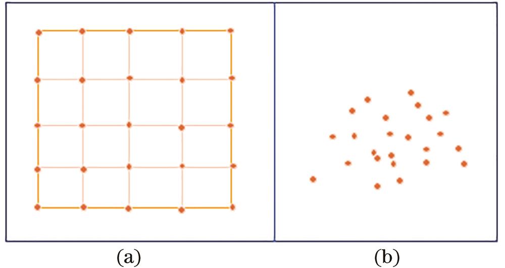
Fig. 1. Comparison schematic of regular 2D image and point cloud. (a) Image grid; (b) point cloud

Download full size

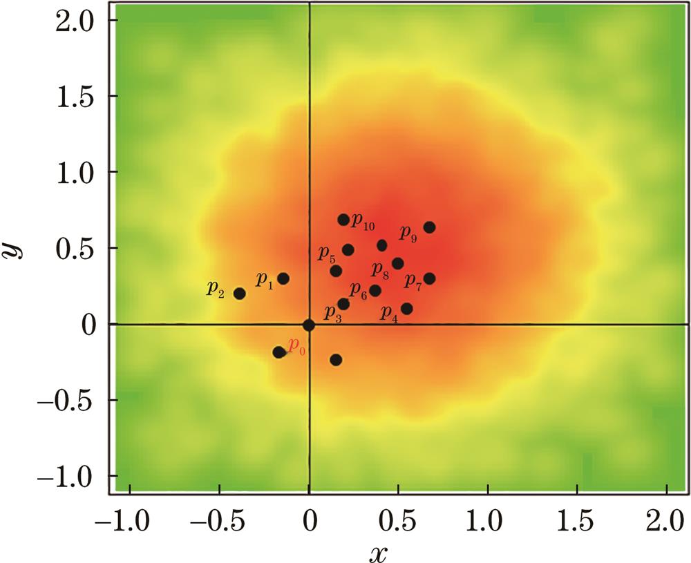
Fig. 2. Schematic of point cloud in local area

Download full size

Fig. 3. U-Net(PointConv) schematic of semantic segmentation of point cloud

Download full size

Fig. 4. Schematic of attention mechanism module structure

Download full size

Fig. 5. Point cloud convolutional network based on attention mechanism (PCNNAM)

Download full size

Fig. 6. GML_DataSetA. (a) Schematic of training set; (b) schematic of test set

Download full size

Fig. 7. Classification results of test set under different networks and the real distribution diagram of GML_DataSetA data set

Download full size

Data set	Ground	Building	Tree	Low vegetation	All
Train set	557142	98244	381677	35093	1072156
Test set	439989	19592	531852	7758	999191

Table 1. All kinds of point cloud distribution in GML_DataSetA training set and test set

Class	Ground	Building	Tree	Low vegetation
Ground	428997	2228	6862	1900
Building	4499	11748	2540	805
Tree	26975	5210	497374	2293
Low vegetation	2539	591	3283	1345
Precision	0.975	0.60	0.935	0.173
Recall	0.927	0.594	0.975	0.212
F1 score	0.950	0.597	0.955	0.191

Table 2. Confusion matrix of classification results in test set obtained by PCNNAM

Parameter	None	$α$ =1.1	$α$ =1.2	$α$ =1.3	$α$ =1.4	$α$ =1.5
Overall accuracy	0.874	0.860	0.940	0.912	0.911	0.788
Overall F1 score	0.487	0.487	0.673	0.559	0.597	0.468

Table 3. Classification results under different coefficients for class balance

Method	Density weighted	Attentional mechanism	F1 score				OA	Average F1 score
Method	Density weighted	Attentional mechanism	Ground	Building	Tree	Low vegetation	OA	Average F1 score
PointNet++	×	×	0.832	0	0.838	0	0.823	0.417
U-Net（PointConv）	√	×	0.937	0.379	0.908	0.122	0.895	0.587
PCNNAM	√	√	0.950	0.597	0.955	0.191	0.940	0.673

Table 4. Classification results of the GML_DataSetA test set under different networks

Category	Train set	Test set
All	753876	411722
Power line	546	600
Low vegetation	180850	98690
Impermeable surface	193723	101986
Car	4614	3708
Fence	12070	742
Roof	152045	109048
Building surface	27250	11224
Shrub	47605	24818
Tree	135173	54226

Table 5. Distribution of various point clouds in the ISPRS Vaihingen 3D semantic marker benchmark data set

Category	Power line	Low vegetation	Impermeable surface	Car	Fence	Roof	Building surface	Shrub	Tree
Power line	328	1	0	0	0	76	3	2	190
Low vegetation	0	77586	9983	154	528	1137	407	6684	2211
Impermeable surface	0	7159	94183	36	9	223	82	233	61
Car	0	121	113	2439	302	94	4	625	10
Fence	0	729	107	46	1704	289	10	3759	778
Roof	124	1416	126	3	123	95357	683	1450	9765
Building surface	14	642	75	41	50	1826	4611	1596	2369
Shrub	0	3537	214	161	1073	1513	344	11364	6612
Tree	3	844	55	44	257	740	259	5388	46635
Precision	0.699	0.843	0.898	0.834	0.421	0.941	0.720	0.365	0.680
Recall	0.547	0.786	0.923	0.658	0.230	0.874	0.411	0.458	0.860
F1 score	0.614	0.834	0.911	0.736	0.297	0.907	0.523	0.406	0.759

Table 6. Confusion matrix of classification results for ISPRS Vaihingen 3D semantic marker benchmark data set obtained by PCNNAM

Method	F1 score									OA	Average F1 score
Method	Power line	Low vegetation	Impermeable surface	Car	Fence	Roof	Building surface	Shrub	Tree	OA	Average F1 score
UM	0.461	0.790	0.891	0.477	0.052	0.920	0.527	0.409	0.779	0.808	0.590
WhuY3	0.371	0.814	0.901	0.634	0.239	0.934	0.475	0.399	0.780	0.823	0.616
LUH	0.596	0.775	0.911	0.731	0.340	0.942	0.563	0.466	0.831	0.816	0.684
BIJW	0.138	0.785	0.905	0.564	0.363	0.922	0.532	0.433	0.784	0.815	0.603
RIT_1	0.375	0.779	0.915	0.734	0.180	0.940	0.493	0.459	0.825	0.816	0.633
NANJ	0.620	0.888	0.912	0.667	0.407	0.936	0.426	0.559	0.826	0.852	0.693
WhuY4	0.425	0.827	0.914	0.747	0.537	0.943	0.531	0.479	0.828	0.849	0.692
U-Net （PointConv）	0.614	0.834	0.911	0.736	0.297	0.907	0.523	0.406	0.759	0.812	0.663
Propoosed method	0.589	0.809	0.902	0.740	0.319	0.911	0.587	0.435	0.768	0.8124	0.673

Table 7. Comparison of the results of PCNNAM and other experiments published by the ISPRS Vaihingen 3D semantic markup competition

Liyuan Wang, Lihua Fu. Airborne LiDAR Point Cloud Classification Based on Attention Mechanism Point Convolutional Network[J]. Laser & Optoelectronics Progress, 2022, 59(10): 1028007

Download Citation

Set citation alerts for the article

Tools

Set citation alerts for the article

Save the article for my favorites

Paper Information