
Felipe Guzmán, Jorge Tapia, Camilo Weinberger, Nicolás Hernández, Jorge Bacca, Benoit Neichel, Esteban Vera. Deep optics preconditioner for modulation-free pyramid wavefront sensing[J]. Photonics Research, 2024, 12(2): 301
- Photonics Research
- Vol. 12, Issue 2, 301 (2024)
Abstract
1. INTRODUCTION
The optics of a wavefront sensor (WFS) aim to modify the optical field such that the integrated intensity field at the detector can be used to infer the phase of the incoming wavefront. This is the case of the Shack–Hartmann WFS (SHWFS)–the workhorse of WFSs [1] widely used in astronomy [2] and ophthalmology [3], which samples the pupil plane by an array of microlenses that are then imaged onto a detector array, where the displacements of the imaged local point spread functions (PSFs) are proportional to the local slopes of the wavefront. Nonetheless, limitations of the SHWFS [4] in terms of sensitivity and phase resolution have prompted the development of a novel family of WFSs that work in the Fourier plane [5], and among them, the pyramid wavefront sensor (PWFS) [6]. The PWFS samples the complex PSF by a four-sided pyramid that projects four versions of the pupil onto the detector array, where the slopes of the wavefront, as well as the phase, can be computed per pixel.
WFSs are at the core of adaptive optics (AO) systems [7], where the PWFS stands out, thanks to its exquisite sensitivity and superb performance, being already tested in current AO systems for large telescopes (8–10 m in diameter) [8,9] in demanding instruments for exoplanet hunting, for instance, making it an ideal candidate to serve novel AO systems in future extremely large telescope projects (25–40 m in diameter) [10]. Nevertheless, despite its great sensitivity, the PWFS has a limited linear response, which must be counteracted by the addition of beam modulation at the expense of a diminished sensitivity. This problem is known as the trade-off between sensitivity and linearity (or sd factor) and has been extensively studied for Fourier-based WFSs [5].
With the growing popularity of deep learning (DL) [11], techniques based on convolutional neural networks have been proposed to improve the inference process of a variety of WFSs [12–16], including the PWFS [17], where the linearity can also be extended with varying degrees of success. The main caveat, though, is that deep neural nets are not very flexible to changing conditions related to real atmospheric turbulence, requiring massive data sets to improve its generalization ability [12], plus forcing the training of a new model for each change in either modal base length, resolution, or modulation, among others.
Sign up for Photonics Research TOC. Get the latest issue of Photonics Research delivered right to you!Sign up now
On the other hand, novel DL applications in computational imaging have incorporated trainable optical elements into optical sensing architectures, which are physically modeled within a neural network, where they can be optimized through an end-2-end (E2E) optimization framework [18,19]. This approach, also known as deep optics, has shown successful results in the design of optimized coded apertures and diffractive elements for novel spectral imaging sensors [20].
In the search for improving the PWFS dynamic range while trying to maintain its sensitivity goodness without the need for modulation, in this work, we seek to incorporate a diffractive element into the optical path of the PWFS that can be trained by taking into account the reconstruction method through an E2E scheme. Even though in the literature there has already been an attempt to replace dynamic modulation by incorporating a diffusing plate in an intermediate pupil plane [21,22], in our initial exploration we propose to place the designed diffractive optical layer at a conjugate Fourier plane before the pyramid, maintaining its classification as a Fourier-plane WFS. This choice might become advantageous, since Fourier-plane WFSs, such as the PWFS, offer fewer noise propagation issues, in contrast with pupil plane WFSs such as the SHWFS [23,24].
Thus, the E2E design process for the new deep PWFS (DPWFS) incorporates the optical propagation model for the PWFS plus the diffractive layer up to the detector. Although any phase recovery algorithm can be used to retrieve the phase out from the intensity measured by the detector, including deep neural nets, we only consider the standard least-squares modal reconstruction, since it is a well-known method used by the AO community. Then, by using the overall modal/phase reconstruction error as the optimization goal, the diffractive optical layer is updated by backpropagating the error. As a result, the diffractive layer of the DPWFS finally acts as an optical preconditioner that can improve the performance of the PWFS forward model and linear reconstruction combination, extending the linear range of operation.
A clear potential advantage of the new approach is that it can improve a current PWFS by only adding the diffractive element at the proper position into the optical path, without changing the operational and calibration procedures already performed in current systems. The designed system has been extensively tested in simulations and also experimentally validated in the PULPOS optical bench [25], where the results show that the performance of a traditionally modulated PWFS can be achieved by the proposed DPWFS without the need for modulation.
2. THEORY
A. Monochromatic Pyramid Wavefront Sensing
Any nonmodulated PWFS system can be generalized by the optical setup shown in Fig. 1. This scheme is divided into three planes by optical transformations: the pupil plane—where the wave is filtered by the telescope aperture and then is focused; the Fourier plane—where the pyramidal prism is placed; and the sensing plane—where the measurement is taken by a focal-plane array.
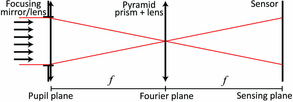
Figure 1.Simplified optical scheme for pyramid Fourier-based wavefront sensing.
The incoming electromagnetic wave can be described as
The PWFS is a special case of , designed by Ragazzoni [6] as a generalization of the Foucault’s knife-edge test. It is a transparent squared pyramid with an apex angle , where each quadrant imposes a local tip/tilt phase in order to split the focused beam into four subpupils. Figure 2 shows examples of the pyramid phase with different values of , along with their respective intensity distribution at the sensing plane, obtained as
![]()
Figure 2.(a)–(c) Pyramids simulated with different values of
The PWFS uses an angle such that the projected subpupils are not overlapped, such as in Fig. 2(f). To simplify the notation, we define as the measurement of the PWFS for a wave with an arbitrary phase . The recovery of from is an inverse problem that can be solved by optimization algorithms such as least squares using the interaction matrix, as will be further explained in Section 3.A.1.
Nevertheless, the PWFS has shown to have great sensitivity, though it has a very limited linear range. The sensitivity/linearity trade-off has been thoroughly analyzed in the literature, and this relationship is further expanded in Section 2.B. In Ref. [6], Ragazzoni proposed to enhance the linear response of the PWFS by modulating the incoming wavefront around the apex of the pyramid. A measure for the modulation is often denoted by , where is the diameter of the projected subpupil and is the number of times the diffraction-limited PSF fits into the modulation radius . Beam modulation as an optical transformation can be modeled as follows:
In summary, the modulated PWFS acquisition can be represented as
B. Sensitivity and Linearity
The desired goal for any WFS design is to have a great sensitivity and a large linear response (or dynamic range). As presented in Ref. [5], they can be computed as
3. DIFFRACTIVE OPTICAL LAYER
The PWFS provides a great sensitivity at the expense of a very limited linearity range. As explained before, the dynamic range can be extended by either oscillating the pyramid [6] or by using a tip/tilt mirror (TTM). Besides sacrificing sensitivity in the process, active modulation poses great problems, such as additional optical alignment and calibration, TTM-to-sensor synchronization, moving parts lifetime, and an extended optical path.
This fact motivates the rationale behind this work, where we want to change the modulation function M for a passive, temporal-independent optical transformation, defined as
We believe that a well-designed can lead to a superior optical transformation that can manage the trade-off between sensitivity and linearity without the need for additional active optical elements.
A. Optical Design
We can design the diffractive optical element through a data-driven E2E training strategy, as depicted in Fig. 3. To achieve this, we use a data set of known incoming wavefronts generated with a variety of real turbulence conditions. Our initial strategy relies on using a turbulence range where the nonlinearity of the PWFS becomes more evident. By simulating the physical propagation, each wavefront is measured by the particular instance of the DPWFS—comprising the optical transformation , that includes , plus the detector—generating an output image from the detector. Then, we solve the respective inverse problem, calibrating the particular instance of the DPWFS to generate the Zernike modal phase estimates, which are used to compute the estimation error through a given loss function. Then, by backpropagating the loss, we can update the discretized optical layer using a classical neural net optimizer such as gradient descent. Thus, every discretized portion of can be considered as a weight of the physical optical neural network, where the amplitude and/or phase can be potentially updated in proportion to the computed error. The whole E2E training process is repeated until convergence is reached.
![]()
Figure 3.DPWFS E2E sensing and reconstruction scheme. An arbitrary phase map of a turbulence profile enters the simulated optical system with the optical layer DE in the forward pass of the DPWFS. Then, a linear estimation of the phase is performed with the pseudo-inverse of the system matrix. The loss function is computed with the error between the Zernike coefficient estimation and the Zernike decomposition of the known phase map. Finally, the error is backpropagated to update each pixel of the DE.
To finish with a physically realizable optical layer , we need to constrain the solution of the optimization to ensure that is always a passive phase element. Therefore, the amplitude of is constrained as
To alleviate the degrees of freedom and ease the simulation of the forward model, we decided to fix the location of within the DPWFS at a conjugate Fourier plane to the tip of the pyramid. In this way, the programmable optical DE can be thought of as an optical preconditioner to the pyramid in the PWFS, so it could even be placed on top of the pyramid if printed in an optical diffractive material [27] or jointly displayed in a spatial light modulator (SLM), as in the digital PWFS implementation [28].
Note that the linear model block in Fig. 3 can be substituted with deep neural networks, such as CNNs [12], to extract the incoming wavefront (either phase or modes) from measured intensities. However, in this work, we focus on using traditional modal least-square inversion of the system matrix, which is also the mainstream method currently adopted by the AO community. Consequently, the only element of the DPWFS being optimized is the optical layer , which indeed works as a preconditioner to the inversion of the linear system matrix.
1. Least-Squares Phase Estimation
We can map the input wavefronts and the measured intensities by creating a linear model based on some orthogonal basis such as Zernike or Karhunen–Loève. For this work, we focus on the Zernike basis, considering a Zernike approximation of an incoming phase such as , where are the normalized Zernike coefficients and is the weight vector. Thus, we build the system or interaction matrix (IM) by concatenating the detector’s intensity response for each Zernike mode as
2. End-2-End Optimization
Considering that DE is the only learnable element in the forward model , the proposed E2E optimization scheme consists in solving the following optimization problem:
During training, the gradients are responsible for updating the values of the DE parameters following the chain rule,
4. RESULTS AND DISCUSSION
A. Data Generation and Training
The E2E model shown in Fig. 3 is implemented in PyTorch, based on the OOMAO toolbox [29] for the physical modeling of the PWFS/DPWFS forward propagation up to the detector. For training and testing, we use the Kolmogorov/von Karman model [30] to generate synthetic phase maps for different levels of turbulence defined by , as implemented in OOMAO. Our baseline resolution is with a sensing subsampling of . Our strategy to enforce a larger dynamic range was to train the DE of the DPWFS using turbulence samples beyond the linear response of the unmodulated PWFS. For training, we randomly generated 10,000 phase maps with different amounts of turbulence levels within two ranges, to 40 (DWPFS-R1) and to 20 (DWPFS-R2). The phase decomposition is performed with 22 Zernike modes without pistons (modes 2–23 under Noll’s sequence). Although using more Zernike modes may lead to better performance, in our case it also leads to an increased computational load during the training process, since the size of the system matrix that must be computed at every iteration is proportional to the number of Zernike modes. Therefore, while also knowing that most of the turbulence energy is concentrated into low-order Zernike modes, we limit the simulation resolution and number of Zernike coefficients, reducing the number of floating-point operations in the GPU and the number of gradients to be computed and stored, preventing VRAM saturation.
Typical values at visible wavelengths for a good place in Europe range within 4–6 cm [31], while a good place in northern Chile often ranges within 10–20 cm [32]. If we consider a telescope of 1.5 m, it leads to an overall range between 7.5 and 38. Therefore, for testing we generated phase maps on demand for an extended range between and 50, while decomposing the phase maps using 66 Zernike modes. In this way, we test for the generalization ability of the system in terms of both turbulence strength and phase resolution.
Every iteration starts by computing the new system matrix using an amplitude of 0.1 for the Zernike coefficients, where the PWFS is often calibrated for maximum sensitivity at low turbulence levels. Then, every training input phase map is propagated through the physical forward model, and the measured image is used to compute the estimated Zernike coefficients obtained by the least-squares algorithm. Once calculating the RMSE between the estimated and ground-truth Zernike coefficients, we can update the optical layer through the backpropagation process offered by PyTorch. The optimizer of each pixel in the DE is updated using decoupled weight decay regularization (AdamW) [33], a stochastic optimization method that decouples the weight decay in the gradient step of a traditional ADAM regularizer [34]. The number of epochs was set to 120, and the initial learning rate was set to . Processing the 10,000 phase maps per epoch takes about 15 min in our desktop computer loaded with an Nvidia RTX2080TI GPU, leading to a design time of nearly 30 h for every DPWFS version.
B. Simulation Results
1. Plain Training
We train the first instance of the DPWFS without noise in the measurements. We train with a very strong turbulence range, to 40 (DWPFS-R1), forcing the DE to adapt to a region where the unmodulated PWFS is clearly within the nonlinear regime, as seen in the dotted red line in Fig. 4. In fact, the nonmodulated PWFS only provides accurate estimations below .
![]()
Figure 4.Estimation performance results using noiseless measurements for a variety of turbulence strengths. The PWFS at different modulation levels is compared with the DPWFS-R1 trained without noise. Each data point is the mean of 10,000 realizations.
Estimation results when testing with an even wider turbulence range (1 to 50 ), in contrast with the training, are shown in Fig. 4. When comparing the nonmodulated PWFS and the optically preconditioned DPWFS, we can clearly observe that the error is vastly diminished within and even beyond the training regime, and it is still competitive for very weak, untrained turbulence regimes, where the PWFS often excels.
We compare the results with the performance of the PWFS with and without modulation, being PWFS-M0 the nonmodulated version, while PWFS-M1, PWFS-M2, or PWFS-M3 is the PWFS modulated with , , or , respectively. When testing with beam modulation applied to the measurement process of the PWFS, we can note, as expected, that modulation is useful to dramatically extend the linear range of the PWFS. Nevertheless, the DPWFS-R1 outperforms the PWFS with or without modulation up to at all turbulence levels and resembles the performance of the PWFS-M3. Note that the DPWFS-R1 was able to improve the performance of the unmodulated PWFS-M0 even beyond the training turbulence regime.
Now, we proceed to check the overall performance of our proposed optical preconditioner in terms of sensitivity , linearity , and SD factor , obtained according to Eqs. (9)–(11), respectively [5]. The comparison results between the DPWFS and the original PWFS for different modulations are presented in Fig. 5. We can observe that the sensitivity is lower for the DPWFS on the low-order Zernike modes, nearly matching the largely modulated PWFS at . On the other hand, for high-order modes, the sensitivity is slightly increased for the DPWFS in contrast to the PWFS.
![]()
Figure 5.Comparison results for the sensitivity
When analyzing the linearity, we can observe that the DPWFS-R1 provides an overall improvement for the whole range of spatial frequencies, in contrast with the unmodulated PWFS and the PWFS with of modulation. Overall, the DPWFS-R1 mostly matches the PWFS-M2, only decreasing its performance for very low spatial frequencies. Finally, the combined metric shows that the DPWFS-R1 performs a bit worse on the low-order modes, while at higher-order modes, beyond radial order 5, it starts to become superior to the PWFS. The mixture of features in terms of sensitivity and linearity shows that the DPWFS-R1 is actually acting as a PWFS that has been modulated.
2. Closed-loop AO Simulation
We performed a simulation to validate the usefulness of the proposed DPWFS in an AO application under realistic turbulence conditions. We generated a sequence of turbulent phase patterns at sampled at 250 Hz, considering a telescope size of 1.5 m and a Fried parameter close to . The results comparing the closed-loop performance for noiseless measurements of the PWFS with and without modulation against the DPWFS-R1 are depicted in Fig. 6.
![]()
Figure 6.Simulation of a closed-loop AO system with a turbulence strength of
At this turbulence strength, we can barely close the AO loop with the unmodulated PWFS, while we can comfortably close it with the DPWFS-R1, which can even adapt faster than the PWFS-M2, which corroborates that the amount of passive modulation achieved by the DPWFS-R1 is larger than . Even though the PWFS-M2 can approach the estimation performance in the closed loop of the DPWFS-R1, in the inset of Fig. 6 we can observe that the final reconstructed PSF achieves a larger Strehl ratio, over 0.28 (DPWFS-R1) in contrast with 0.23 (PWFS-M2).
3. Testing with Noise
We added noise to the measurements to understand its impact on the performance of the PWFS and DPWFS. For that, we simulate both photon and readout noise. The photon noise is modeled as a Poisson distribution as follows:
Figure 7 shows the performance results obtained when considering noisy measurements using parameters of , , and . Now, the PWFS without modulation is barely affected by noise, in contrast with the DPWFS-R1, which is clearly affected at weak turbulence, which in fact correlates with the sensitivity issues reported in Fig. 5. Nevertheless, and despite being very close in terms of sensitivity, the performance for the DPWFS-R1 is always superior to the PWFS modulated at , keeping a great performance at higher turbulences.
![]()
Figure 7.Estimation performance results using noisy measurements for a variety of turbulence strengths. We added readout noise with
We devise two possible approaches to handle noise and perhaps increase the sensitivity at the potential expense of a slight loss of linearity. First, we may believe that the turbulence range used to train the DPWFS-R1 was too strong, so there was a loss of attention to the small turbulence regime. Also, we may also think that using an extended range would be best; however, optimizing over the full range of turbulence was not as effective, leading to worse results over the whole range. Therefore, we train a new version of the DPWFS using noiseless measurements at a softer turbulence range within to 20 (DWPFS-R2). Second, we also know from the neural network literature [35] that adding noise to the training process has a regularization effect. By decreasing the possibility of overfitting the training data, training with noise should increase the robustness of the trained optical layer. Therefore, we retrain the DPWFS-R1 using its original turbulence range but now using noisy measurements (DPWFS-N1), affected solely by readout noise with .
4. Training with Alternative Turbulence Range
In this case, we are going to explore whether or not training the DPWFS with a moderate turbulence range may improve its robustness to noise. The DPWFS-R2 is trained with a turbulence range within to 20 and noiseless measurements. We can observe the performance of the new DE under noise in Fig. 7, where we can notice a better immunity to noise at weaker turbulence levels, improving over the former DPWFS-R1 and being as competitive as the unmodulated PWFS. However, we can also notice that the improvement of the DPWFS-R2 at strong turbulence is not as solid as the DPWFS-R1 or the PWFS-M3, although it is still noticeably better than the PWFS without modulation, resembling what is expected for the PWFS at a lower modulation level, as seen in former Fig. 4.
As shown in Fig. 8, it is interesting to note that the sensitivity of the DPWFS-R2 is able to outperform the DPWFS-R1 and even the PWFS-M3, which corroborates its good performance at very weak turbulence levels. Nonetheless, the PWFS-M0 is unbeatable at the lowest orders. On the contrary, the DPWFS-R2 loses a bit of linearity, in contrast with the DPWFS-R1, though it is still superior to the PWFS without modulation.
![]()
Figure 8.Comparison results for the sensitivity
5. Training with Noise
Given the former results for noisy measurements, we also explore whether or not training the DPWFS with noise improves its robustness. In this opportunity, we train a new DE with the same original data set for DWPFS-R1—with turbulence from to 40—with the addition of readout noise of to the measurements. We can observe the performance of the DPWFS-N1 in Fig. 7, where we can notice a better immunity to noise at weaker turbulence levels, improving over the former DPWFS-R1 and being more competitive to the PWFS-M0, though not as close as the DPWFS-R2. However, we can also notice that the improvement in dynamic range at large turbulence levels of the DPWFS-N1 is not as strong as the noiseless DPWFS-R1, though it is only slightly worse than the PWFS-M3 and noticeably better than the DPWFS-R2. Overall, the DPWFS-N1 is much better than the PWFS without modulation at all turbulence levels beyond .
It is worth noting that when comparing the sensitivity shown in Fig. 8, the DPWFS-N1 acts very similar to the DPWFS-R2, always better than the DPWFS-R1 and the PWFS-M3. On the other hand, the DPWFS-N1 only sacrifices a bit of the linearity advantages offered by the DPWFS-R1, being slightly better than the DPWFS-R2 while still being fairly superior to the PWFS without modulation. The sd analysis is very correlated to the reported performance results, where training with noise finally sacrifices some dynamic range in exchange for a better immunity to noise at weak signals.
6. Noise Analysis
We analyze the performance of the DPWFS-R1 and DPWFS-N1 under different noise conditions, simulating noisy measurements for combinations of readout and photon noise statistics at four fixed turbulence regimes. The results are displayed in Fig. 9.
![]()
Figure 9.Performance results for different combinations of photon and readout noise statistics. Each colored surface represents the RMSE fluctuations for the unmodulated PWFS, DPWFS-R1, and DPWFS-N1. Every plot represents a fixed turbulence regime. (a)
Overall, we can see that the PWFS is very robust to a variety of noise distributions, showing a plain distribution for the different turbulence strengths. This is expected, since the PWFS-M0 has the best overall sensitivity in our metrics, as shown in Figs. 8 and 5. Also, both trained DPWFS versions are more affected by noise, although the DPWFS-N1 is clearly more robust to readout noise, since it was trained for that.
For the low turbulence test shown in Fig. 9(a), we can notice that the PWFS is superior overall, unless for very low noise situations. Although the DPWFS-N1 offered better immunity to readout noise than the DPWFS-R1, it seemed slightly more affected by photon noise.
Starting at mid-turbulence levels as shown in Fig. 9(b), we can start to see the benefits of training with noise, where the DPWFS-N1 is always better than the PWFS-M0. For higher turbulence levels, as seen in Figs. 9(c) and 9(d), readout noise becomes less of an issue, while photon noise seems more harmful to the performance, though the gains in dynamic range for both DPWFSs are more evident and relevant compared with the noise. Nonetheless, the noise seems to impact the potential improvement in linearity.
7. Diffractive Elements
The resulting DEs after 120 epochs of training for all the versions of the DPWFS are shown in Fig. 10. Note that for DPWFS-R1, trained for the range between and 40 without noise, we obtained the DE displayed in Fig. 10(a), where we can clearly observe a cross shape in the middle section, which will tend to soften the hard edges of the pyramid once overimposed. This cross pattern helps in distributing the light within neighboring pyramid faces, somehow partially emulating the modulation effect. We can also see that the cross shape lies within a circular pattern, which coincides with the area covered by most of the energy of the projected PSFs on top of the pyramid apex for the given turbulence range. Overall, the rest of the diffractive patterns are just the result of the backpropagation and most likely may only play a significant role for stronger turbulence, redirecting light toward the center.
![]()
Figure 10.DE training results after 120 epochs. (a) Phase distribution of the DPWFS-R1 DE trained without noise; (b) phase distribution of the DPWFS-R2 DE trained without noise; (c) phase distribution of the DPWFS-N1 DE trained with readout noise of
The resulting DE for the DPWFS-R2 trained with the turbulence range within to 20 can be seen in Fig. 10(b), where we can observe a noticeable difference from the previously trained DPWFS-R1 shown in Fig. 10(a), now displaying more high-frequency patterns toward the center of the diffractive layer area. Nevertheless, the cross shape is thinner but still visible in the center, although the radius of the circular area is smaller, coinciding with the smaller area illuminated by the PSFs originating from weaker turbulence regimes. Please note the presence of strong diagonal patterns beyond the central circular area, which would most likely redirect light toward the projected pupils for stronger turbulence than the ones used for training.
Finally, the resulting DPWFS-N1 DE trained for the range between and 40 with noise can be seen in Fig. 10(c), where we can observe similarities and differences from the DPWFS-R1 DE previously trained without noise [shown in Fig. 10(a)]. On the one hand, the DE for DPWFS-N1 displays fewer high-frequency features within the diffractive pattern area, in contrast with the DPWFS-R1, practically erasing portions of the diffractive features beyond the central circular area. On the other hand, the cross shape in the middle of the diffractive area remains very similar.
After training, the net effect of all the DEs is redirecting light trying to better distribute light between the subpupils, counteracting the natural behavior of the pyramidal prism without modulation—although this always will come at the expense of a loss of sensitivity despite the evident gains in linearity.
8. Training in the Pupil Plane
We are aware that there were previous efforts to use passive optical modulation in exchange for active optical modulation in PWFSs [21,22]. Nonetheless, since the original attempt was through the addition of a diffuser plate at the pupil plane, we also want to explore what is the effect of training a diffractive layer in the pupil plane instead of the Fourier plane.
For that, we use the exact same training data and E2E optimization procedure previously used for training DPWFS-R1, but now we are placing the diffractive element at the pupil plane (PUPIL-R1). Performance results in noiseless measurements are shown in Fig. 11 (continuous lines), where we can notice that either training in the Fourier plane or the pupil plane can achieve very similar results, demonstrating an equivalent improvement in the dynamic range, in contrast with the unmodulated PWFS-M0, although the DPWFS-R1 is always superior to the PUPIL-R1.
![]()
Figure 11.Training results for different levels of turbulence. The continuous lines represent the testing of each turbulence profile without noise, and the segmented line is with the same phase but now with
Now, when testing with noise (dashed lines), we can corroborate that the unmodulated PWFS is barely affected, and mostly at low turbulences. On the other hand, both DPWFS-R1 and PUPIL-R1 are more impacted by noise, especially at weak turbulence. Although both Fourier and pupil plane versions are able to increase the dynamic range for strong turbulence regimes, PUPIL-R1 results are less robust than DPWFS-R1, overall.
C. Experimental Validation
1. Optical Implementation
We perform a proof of concept for the proposed DPWFS using the PULPOS optical bench [25], which has been envisioned to provide multiple branches to simultaneously test a variety of novel WFS ideas. In this case, the branch of PULPOS used in this experiment is depicted in Fig. 12. We use a fiber-coupled laser source (Thorlabs S1FC635) attached to an air-spaced doublet collimator (Thorlabs F810APC-635) and a beam expander (Thorlabs GBE02-A, ). The beam is spatially filtered by a 5 mm diameter aperture stop (AS). Then, the beam passes through a 4f-system with 1× magnification (composed by and ) and a beam splitter (), being projected onto a reflective high-speed SLM (, Meadowlark HSP1920-488-800-HSP8) positioned at a conjugate pupil plane of the system to imprint the phase maps that emulate the desired turbulence. Then, light is redirected by toward another magnification 4f-system (composed by and ) that reaches lens (400 mm) to focus the beam, generating a Fourier plane.
![]()
Figure 12.Optical setup to implement the digital PWFS or the designed DPWFS at the PULPOS AO bench.
To ease the experimental calibration and be able to test either a PWFS or the newly designed DPWFS, we opted to implement the digital PWFS [28] using a second SLM. Therefore, we placed (Thorlabs EXULUS-4K1, , 400–850 nm, 3.74 μm pixel size) at the Fourier plane. By projecting the digital pyramid diffraction pattern in , we use lens (200 mm) to image the subpupils onto a high-speed CMOS camera (Emergent Vision HR-500-S-M, 9 μm pixel size, 1586 frames per second). Then, we can easily swap the phase pattern projected onto to display the DPWFS instead, which is a combination of the digital PWFS plus the designed DE. In this case, we use the robust version trained with noise, DPWFS-N1, as shown in Fig. 10(c).
2. Experimental Results
We use the exactly same test data set used in the simulations, comprising 100 randomly generated phase maps for a variety of turbulence strengths between and . Before testing the PWFS or DPWFS, we obtain the respective system matrix using the first 65 Zernike coefficients (without considering the piston). The calibration was made using an amplitude of 0.25 applied to the Zernike coefficients, which is slightly larger than the simulated amplitude of 0.1. The reason was that the limited dynamic range of 8-bits provided by the generated issues in the computed system matrices. Note that all measurements were cropped using a circle mask at the center of the detector—with the same size as any of the projected pupils—to eliminate the zeroth-order diffraction produced by the diffractive digital pyramid, as suggested in Ref. [28]. Then, we can test any of the systems by sequentially projecting the test phase maps and computing the RMSE between the ground truth and the estimated coefficients.
We tested the unmodulated pyramid PWFS-M0 and then repeated the test for a modulation of (PWFS-M2), which was digitally implemented in the same by adding a proportional tip/tilt to the PWFS pattern. We took and then integrated 20 snapshots of equally spaced tip/tilt positions in the unitary circle to emulate the desired beam modulation. Both versions of the PWFS are tested against the designed DPWFS-N1. Results can be seen in Fig. 13, where the DPWFS-N1 presents a balanced performance overall in the whole range of turbulence tested, only being slightly surpassed by the unmodulated PWFS at extremely weak turbulence (see inset) and the PWFS-M2 at strong turbulence.
![]()
Figure 13.Experimental performance results comparing the unmodulated pyramid PWFS-M0, the modulated pyramid at
The overall behavior of the DPWFS-N1 closely follows the modulated PWFS-M2 above turbulences of in terms of average trend and standard deviation. Nonetheless, the DPWFS-N1 shows better immunity to noise at weaker turbulences, even though it was never trained for that regime. Please note, though, that the PWFS-M2 shows a smaller standard deviation at low turbulences because (see inset) the digital modulation was captured in several measurements, naturally filtering noise by averaging. Nonetheless, it should be noted that the advantages offered by both the DPWFS-N1 and the modulated PWFS-M2 diminish as the turbulence gets stronger. This effect might be produced also by dynamic range issues of the turbulent phase maps projected onto that start suffering from severe wrapping and undesired diffraction effects.
5. CONCLUSION
The PWFS is a very sensitive device but is also highly nonlinear, with a limited dynamic range. Although linearity can be extended by using dynamic optical modulation, it comes at the expense of a diminished sensitivity plus the need for active optical devices. In this work, we proposed to exchange active optical modulation by including a designed passive diffractive element into the optical path of the PWFS, specifically placed at a conjugated Fourier plane where the tip of the pyramid lies. This DE can be considered as an optical layer that can be designed under the paradigm of deep optics, using the same tools used for the training of artificial neural networks. To design the novel DPWFS, we developed an E2E simulation framework to train the DE, which includes the physical propagation model of the DPWFS and a traditional least-squares modal phase estimation model. In this way, the DE can be trained using a collection of training data sets comprising pairs of input phase maps and the desired output Zernike coefficients to be estimated. Then, the DE acts as an optical preconditioner to the linear inversion.
We devised a strategy to extend the dynamic range of the DPWFS by training with data sets of strong turbulence phase maps where the PWFS is clearly in the nonlinear regime. Simulation results with a large range of turbulence conditions showed a noticeable improvement in the dynamic range equivalent to over of modulation when using the optically preconditioned DPWFS for strong turbulences, while approaching the estimation performance of the unmodulated PWFS at weak turbulences. Nevertheless, the analysis indicated that the DPWFS presented a loss in sensitivity equivalent to the modulated PWFS at high modulation, while the gain in linearity was following the behavior of a modulated PWFS at low modulations. This analysis was validated once testing the DPWFS under noisy measurements, where the unmodulated PWFS is very robust to noise, while the modulated versions of the PWFS or the DPWFS were not as good, although the DPWFS was not as affected as the PWFS with of modulation. Moreover, we tested the performance of the DPWFS in a simulated AO experiment for a strong turbulence near the limit of the training regime (), reinforcing the fact that the DPWFS is even more effective than a modulated PWFS at , leading to a faster correction and a better Strehl ratio.
To boost the sensitivity of the DPWFS, we proposed two approaches: training with a range of medium turbulence or training with noisy measurements. Although the two strategies were successful in improving sensitivity, they also diminished the gain in dynamic range in contrast to the original DPWFS. Nonetheless, training the DPWFS with noise seemed a better choice, not only because of the results, but also because it fits the neural network theory in terms that noise can improve the generalization ability of the trained layer and therefore it can become more robust. In an additional simulation, we also demonstrated that we can also train a passive diffractive element that can be placed at the pupil plane of the PWFS, although the Fourier plane version was more effective and robust. This finding is interesting, since the proposed DPWFS can still be considered as a Fourier plane WFS.
We also implemented the digital diffractive version of the PWFS in the PULPOS AO bench, which allowed a fair comparison with the designed DPWFS. Experimental results validated the advantages of using the designed optical layer, where the DPWFS was able to pair the performance of a traditional PWFS with of modulation for strong turbulence while still approaching the nice performance of the unmodulated PWFS at weak turbulence. Although the improvement of the proposed DPWFS was a bit lower than what was seen in the simulations, which can be due to several experimental issues, the reported results are still a clear demonstration that the proposed designed diffractive pattern can effectively extend the dynamic range of the PWFS without sacrificing the performance at weak turbulence regimes, as expected for an equivalent modulation level. Therefore, we can conclude that the DPWFS can effectively act as a PWFS with an improved passive modulator, providing a more advantageous compromise between linearity and sensitivity beyond what active optical modulation may offer.
Designing and adding an optical preconditioner to the PWFS is just the tip of the iceberg. For instance, further work may include the co-design of one or several diffractive optical layers with a deep neural network reconstructor. Thus, the proposed methodology for the DPWFS opens the avenue for the design of new WFSs, not only for demanding astronomical AO, but also for sophisticated AO applications such as space and underwater optical communications, and imaging through scattering media in microscopy [36] and ophthalmology [37].
References
[3] J.-F. Le Gargasson, M. Glanc, P. Léna. Retinal imaging with adaptive optics. C. R. Acad. Sci. IV, 2, 1131-1138(2001).
[7] R. K. Tyson, B. W. Frazier. Principles of Adaptive Optics(2022).
[9] R. Clare, B. Engler, S. Weddell. Numerical evaluation of pyramid type sensors for extreme adaptive optics for the European extremely large telescope. Adaptive Optics for Extremely Large Telescopes, 5(2017).
[11] Y. LeCun, Y. Bengio, G. Hinton. Deep learning. Nature, 521, 436-444(2015).
[17] C. Weinberger, F. Guzmán, J. Tapia. Design and training of a deep neural network for estimating the optical gain in pyramid wavefront sensors. Imaging and Applied Optics Congress, JF1B.6(2022).
[26] G. I. Taylor. The spectrum of turbulence. Proc. R. S. London A, 164, 476-490(1938).
[30] V. I. Tatarski. Wave Propagation in a Turbulent Medium(2016).
[33] I. Loshchilov, F. Hutter. Decoupled weight decay regularization(2019).
[34] D. P. Kingma, J. Ba. Adam: a method for stochastic optimization(2017).
[35] C. M. Bishop. Neural Networks for Pattern Recognition(1995).
[38] https://github.com/FOGuzman/End2EndPyrWFS. https://github.com/FOGuzman/End2EndPyrWFS

Set citation alerts for the article
Please enter your email address
© Copyright 2018-2021 | Chinese Laser Press. All Rights Reserved 沪ICP备15018463号-20