Image-Domain Multimaterial Decomposition for Dual-Energy CT Based on Dictionary Learning and Relative Total Variation

Junru Jiang; Haijun Yu; Changcheng Gong; Fenglin Liu

doi:10.3788/AOS202040.2111004

Journals >Acta Optica Sinica >Volume 40 >Issue 21 >Page 2111004 > Article

Acta Optica Sinica
Vol. 40, Issue 21, 2111004 (2020)

Image-Domain Multimaterial Decomposition for Dual-Energy CT Based on Dictionary Learning and Relative Total Variation

Junru Jiang^1、2、3, Haijun Yu^2、3, Changcheng Gong⁴, and Fenglin Liu^2、3、*

Author Affiliations

¹State Key Laboratory of Mechanical Transmission, Chongqing University,Chongqing 400044, China

²Key Laboratory of Optoelectronic Technology and Systems of the Ministry of Education, Chongqing University, Chongqing 400044, China

³Engineering Research Center of Industrial Computed Tomography Nondestructive Testing, Ministry of Education, Chongqing University, Chongqing 400044, China

⁴College of Mathematics and Statistics, Chongqing Technology and Business University, Chongqing 400067, China

show less

DOI: 10.3788/AOS202040.2111004 Cite this Article Set citation alerts

Junru Jiang, Haijun Yu, Changcheng Gong, Fenglin Liu. Image-Domain Multimaterial Decomposition for Dual-Energy CT Based on Dictionary Learning and Relative Total Variation[J]. Acta Optica Sinica, 2020, 40(21): 2111004 Copy Citation Text

show less

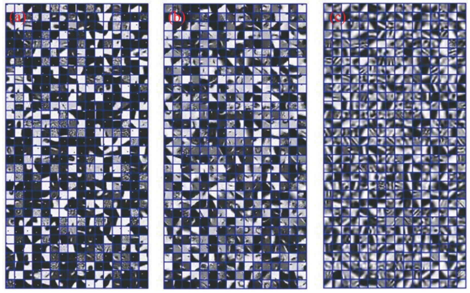
Fig. 1. Dictionaries used in the experiments. (a) Dictionary of physical phantom; (b) dictionary of turtle; (c) dictionary of chicken feet

Download full size

Reconstruction results of mouse thorax phantom by SIRT in high and low energies. (a) High energy reconstruction image; (b) low energy reconstruction image

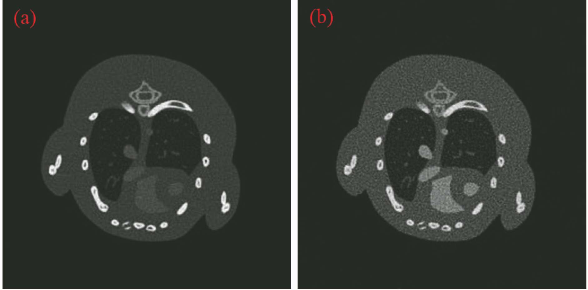
Fig. 2. Reconstruction results of mouse thorax phantom by SIRT in high and low energies. (a) High energy reconstruction image; (b) low energy reconstruction image

Download full size

Fig. 3. Material decomposition results by different algorithms. (a) Bone; (b) soft issue; (c) iodine contrast agent

Download full size

Fig. 4. Reconstruction results of partial turtle projection by PISSC in high and low energies. (a) High energy reconstruction image; (b) low energy reconstruction image

Download full size

Fig. 5. Material decomposition results by different algorithms. (a) Bone; (b) soft issue; (c) air

Download full size

Fig. 6. Magnified ROI area. (a) DIMD; (b) TVMD; (c) DLMD; (d) RTVMD; (e) DL-RTV

Download full size

Fig. 7. Reconstruction results of chicken feet by FBP in high and low energies. (a) High energy reconstruction image; (b) low energy reconstruction image

Download full size

Fig. 8. Material decomposition results by different algorithms. (a) Bone; (b) soft issue; (c) iodine

Download full size

Fig. 9. Magnified ROI area. (a) DIMD; (b) TVMD; (c) DLMD; (d) RTVMD; (e) DL-RTV

Download full size

Input:θ,ε,T,L,K, and other parameters;
Initialization:F⁽⁰⁾=0,V⁽⁰⁾=0,J⁽⁰⁾=0,k=0。
Step1:Train dictionary
1 Reconstruct dual-energy CT images;
2 Acquire original material images using the DIMD;
3 Train a dictionary employing the K-SVD method.
Step2:Decompose materials
0 For k=1:Kdo
1 Update F⁽^k⁺¹⁾ using Eq.(24);
2 Update J, ${α_{m}}_{m = 1}^{M}$ using Eq.(28);
3Update V using Eq.(29);
4 End for;
Output:Material images tensor F.

Table 1. Flow chart of the DL-RTV solution

Item	Material	Method
Item	Material	DIMD	TVMD	DLMD	RTVMD	DL-RTV
RMSE	Bone	0.0345	0.0460	0.0313	0.0337	0.0304
	Soft issue issue	0.1256	0.0975	0.0909	0.0957	0.0854
	I	0.0952	0.0655	0.0687	0.0444	0.0592
PSNR	Bone	29.243	26.752	30.103	29.437	30.353
	Soft issue issue	18.023	20.224	20.826	20.382	21.375
	I	20.430	23.678	23.256	27.057	24.555
SSIM	Bone	0.9612	0.9716	0.9822	0.9855	0.9855
	Soft issue issue	0.7228	0.9193	0.9325	0.9359	0.9364
	I	0.6754	0.9843	0.9755	0.9542	0.9904
FSIM	Bone	0.8860	0.9434	0.9528	0.9534	0.9628
	Soft issue issue	0.6637	0.8822	0.9036	0.8962	0.9040
	I	0.5907	0.9352	0.9312	0.9213	0.9358

Table 2. Quantitative evaluation results of material decomposition by different algorithms

Download Citation

Set citation alerts for the article

Tools

Set citation alerts for the article

Save the article for my favorites

Paper Information