
Yueqiang Zhang, Mingjie Chen, Biao Hu, Wenjun Chen, Yihe Yin, Qifeng Yu, Xiaolin Liu. Transmission Mechanism and Suppression Methods of Measurement Error Based on Camera Networking[J]. Acta Optica Sinica, 2023, 43(21): 2112002
- Acta Optica Sinica
- Vol. 43, Issue 21, 2112002 (2023)
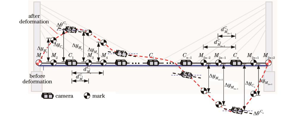
Fig. 1. Schematic diagram of serial camera network based on displacement transmission
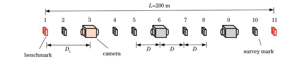
Fig. 2. Sketch map of camera network basic configuration
Fig. 3. Numerical simulation procedure of camera network
Fig. 4. Statistical results of camera network basic configuration. (a) Average value; (b) root mean square error
Fig. 5. Influence of camera station number on transmission error
Fig. 6. Influence of subsidence amplitude and inclination angle on transmission error
Fig. 7. Influence of benchmark position on transmission error. (a) Root mean square error; (b) condition number of survey matrix (color of grid in picture represents magnitude of corresponding dependent variable. Magnitude that color represents corresponds to color bar on right side of picture)
Fig. 8. Influence of distance between camera station and benchmark position (D1) on transmission error. (a) Changing distance between camera station and benchmark position on one side of network; (b) changing distance between camera station and benchmark position simultaneously on both sides of network
Fig. 9. Sketch map of survey mark distribution between camera stations
Fig. 10. Influence of survey mark position on transmission error. (a) Root mean square error; (b) condition number of survey matrix (color of grid in picture represents magnitude of corresponding dependent variable. Magnitude that color represents corresponds to color bar on right side of picture)
Fig. 11. Influence of survey mark number on transmission error
Fig. 12. Relationship between transmission error and error coefficient of camera network. (a) Influence of benchmark position; (b) influence of survey mark position
Fig. 13. Validation experiment of camera network on long-span cable-stayed bridge
Fig. 14. Monitoring results of cable-stayed bridge camera network with different network configurations (Cf1-Cf6 represent network configurations 1-6 respectively in Table 4)
|
Table 1. System parameters of camera network basic configuration
| ||||||||||||||||||||||||||||||||||||||||||||||||||||||||||||||||||||||
Table 2. Comparison of camera network optimization with different camera stations
|
Table 3. Parameters of experimental camera
|
Table 4. Bridge monitoring results of different error suppression methods

Set citation alerts for the article
Please enter your email address
© Copyright 2018-2021 | Chinese Laser Press. All Rights Reserved 沪ICP备15018463号-20