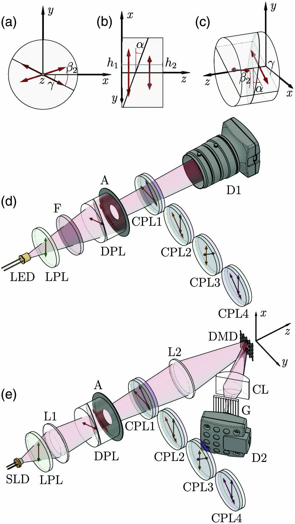
Fig. 1. (a) Front view, (b) side view, and (c) near-isometric view illustration of the quartz-wedge DPL. The parameter α is the wedge angle, β2 is the angle between the optic axes of wedges 1 and 2 having position-dependent thicknesses h1 and h2, respectively, and γ is the orientation angle of the whole DPL. (d) Measurement setup of the polarization Stokes parameters: source LED; LPL, linear polarizer; F, spectral filter; DPL, depolarizer; aperture A; CPL1–4, circular polarizers; D1, camera and objective. (e) Measurement setup of the coherence Stokes parameters. SLD, superluminescent diode; L1 and L2, lenses; DMD, digital micromirror device array; CL, cylindrical lens; G, spectrometer grating; and D2, camera detector array. Other components are the same as in (d).

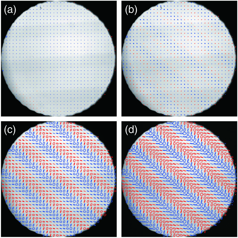
Fig. 2. Measured spectrally integrated polarization properties after the quartz-wedge DPL illuminated by linearly polarized LED light. The polarization state is represented in terms of polarization ellipses: the size indicates the degree of polarization while red and blue colors refer to right-hand and left-hand polarization. The gray background illustrates the intensity distribution. (a) Unfiltered LED spectrum with FWHM of 15 nm. Filtered spectra with FWHMs of (b) 10 nm, (c) 3 nm, and (d) 1 nm.

Fig. 3. Example of measured interference fringes without the DPL. The left column shows the intensity fringes Ii(x′,λ) observed directly on the camera when light is transmitted through polarizer elements (a) CPL1, (b) CPL2, (c) CPL3, and (d) CPL4. (e)–(h) in the right column show the corresponding normalized Stokes-parameter fringes Cn(x′,λ), calculated using the error compensated forms of Eqs. (13)–(16) presented in Appendix B, and Eq. (18).

Fig. 4. Example of the measured interference fringes with the DPL included. The quantities in (a)–(h) are the same as in Fig. 3.

Fig. 5. (a)–(h) Simulated (left) and measured (right) coherence Stokes parameters μn(x1,x2,λ), n∈{0,…,3}, at a single wavelength λ=659.4  nm; (i), (j) electromagnetic degree of coherence μ(x1,x2,λ); (k) measured SLD spectrum; (l) two-axis color map to include the phase information of the complex-valued data. Visualization 1 shows the effect of scanning the wavelength over the spectrum.

Fig. 6. Simulated data. Absolute values (a)–(d) of the coherence Stokes parameters Sn(x,−x,λ) and (e)–(h) of the normalized parameters μn(x,−x,λ); (i)–(l) phase arg[μn(x,−x,λ)]. The line in the bottom-left corner visualizes the input polarization direction. See Visualization 2 for the effect of rotating the direction.

Fig. 7. Illustration of the measured coherence Stokes parameters. The quantities in (a)–(l) are the same as in Fig. 6.