The second-order spatial coherence properties of random electromagnetic light beams of arbitrary spectral bandwidth can be fully characterized by the 2×2 cross-spectral density matrix (CSDM) ^[1]. Alternatively and equivalently, the four-coherence or two-point Stokes parameters, which are extensions of the traditional polarization (one-point) Stokes parameters, could be employed to quantify electromagnetic coherence ^[2–6]. The coherence Stokes parameters of the field at the pinholes of Young’s interferometer are known to determine directly the modulation contrasts and positions of the observed polarization Stokes-parameter fringes ^[4,6], whatever type of polarization-modulating elements are placed in front of the pinholes. This provides a fundamental approach to experimental determination of the coherence Stokes parameters ^[7–9], though other methods are also possible ^[10]. Thus frequency-dependent coherence Stokes parameters can be measured using Young’s two-pinhole experiment with narrowband spectral filtering ^[9] and the type of polarizer-wave plate combinations commonly used in the determination of polarization Stokes parameters.

In this work, we present and characterize a system for measuring the spectral coherence Stokes parameters of broadband light using Young’s interferometer based on a digital micromirror device (DMD) ^[11] and a diffraction grating. In the experiments, we characterize a nontrivial spatially partially coherent and nonuniformly polarized secondary source that consists of a superluminescent diode (SLD) and a quartz-wedge depolarizer (DPL). This source is (nearly) fully polarized at each frequency, yet is essentially unpolarized when the frequency-integrated (or, equivalently, time-domain ^[12]) polarization matrix is considered. This source belongs to the class discussed in Ref. ^[13], except that, despite its relatively narrow spectral bandwidth, it cannot be described as being quasi-monochromatic.

We begin, in Section 2, by recalling the relevant coherence quantities. The primary and secondary light sources used in the experiments are described in Section 3, and a model for their coherence-polarization properties is given. In Section 4, we introduce our measurement system, and in Section 5, we describe the process of extracting the coherence information from camera data. The theoretical and measurement results are compared in Section 6 and possible improvements of our system are discussed in Section 7. Finally, in Section 8, we briefly summarize the work.

Let us consider a random beamlike electromagnetic field with electric-field realizations E(r,λ)=[Ex(r,λ),Ey(r,λ)]T, where Ei(r,λ), i∈{x,y}, are the two transverse components, r=(x,y), λ is the wavelength, and T denotes matrix transpose. The second-order statistical properties of the field in the space-frequency domain are described by the 2×2 CSDM, where the angle brackets and the asterisk stand for ensemble averaging and complex conjugation, respectively. The spectral coherence Stokes parameters are defined in terms of the CSDM elements as ^[2,5] where, explicitly, Wij(r1,r2,λ)=⟨Ei*(r1,λ)Ej(r2,λ)⟩, with i,j∈{x,y}. Setting r1=r2=r, we encounter the traditional polarization (one-point) Stokes parameters, It is often convenient to use the normalized coherence Stokes parameters, where S0(r,λ) is the spectral density (or spectrum) of the field. Further, we define the (real-valued) electromagnetic degree of coherence as ^[4,6] This quantity, like the magnitudes of the normalized coherence Stokes parameters, is bounded in the range 0≤μ(r1,r2,λ)≤1.

To test the measurement system of the coherence Stokes parameters (to be described in detail in Section 4), we constructed a polychromatic secondary source with nontrivial but well-characterized coherence-polarization properties. We used an SLD as a primary source and modulated the polarization state of the emitted light with a Cornu-type quartz-wedge DPL. In what follows, we will refer to the coordinate axes perpendicular and parallel to the junction of the SLD as x and y, respectively. The SLD used in our experiments (Superlum SLD-260-MP) emits radiation at a center wavelength of 670 nm, with spectral full width at half-maximum (FWHM) of 7.5 nm. The light is linearly polarized in the y direction, and the radiation pattern has FWHM divergence angles of 35° and 10° in the x and y directions, respectively.

We first characterized the spatial coherence properties of the SLD alone with the DMD-based Young’s interferometer ^[11]. We found the radiation to be spatially partially coherent along the x axis, indicating multimode operation. Since no detailed information on the cavity structure was available, the true mode structure was unknown. We therefore modeled the beam by fitting the measured spatial coherence distribution into the standard Gaussian Schell model. A good fit was found when the (propagation-invariant) ratio of the spatial coherence width, σ, and the beam width, w, was taken to be σ/w≈1.7, which implies β≈0.79 in the notation of Ref. ^[14]. It is thus convenient to represent the primary source in the x direction (along the x axis, y=0) in the form of a Mercer expansion ^[15]: where ψj,0(x,λ)=ψj,0(x,λ)[0,1]T, with [0,1]T being the unit vector in the y direction. In addition, ψj,0(x,λ) are the usual Hermite–Gaussian laser modes: where Hj(x) is a Hermite polynomial of order j, and wc=wβ. Further, in the notation of Ref. ^[14], the weight factors αj are Inclusion of three lowest-order modes (j=0,1,2) with α1=0.117α0 and α2=0.014α0 is sufficient to represent the SLD beam well. The coherence distribution in the y direction could be analyzed in an analogous manner.

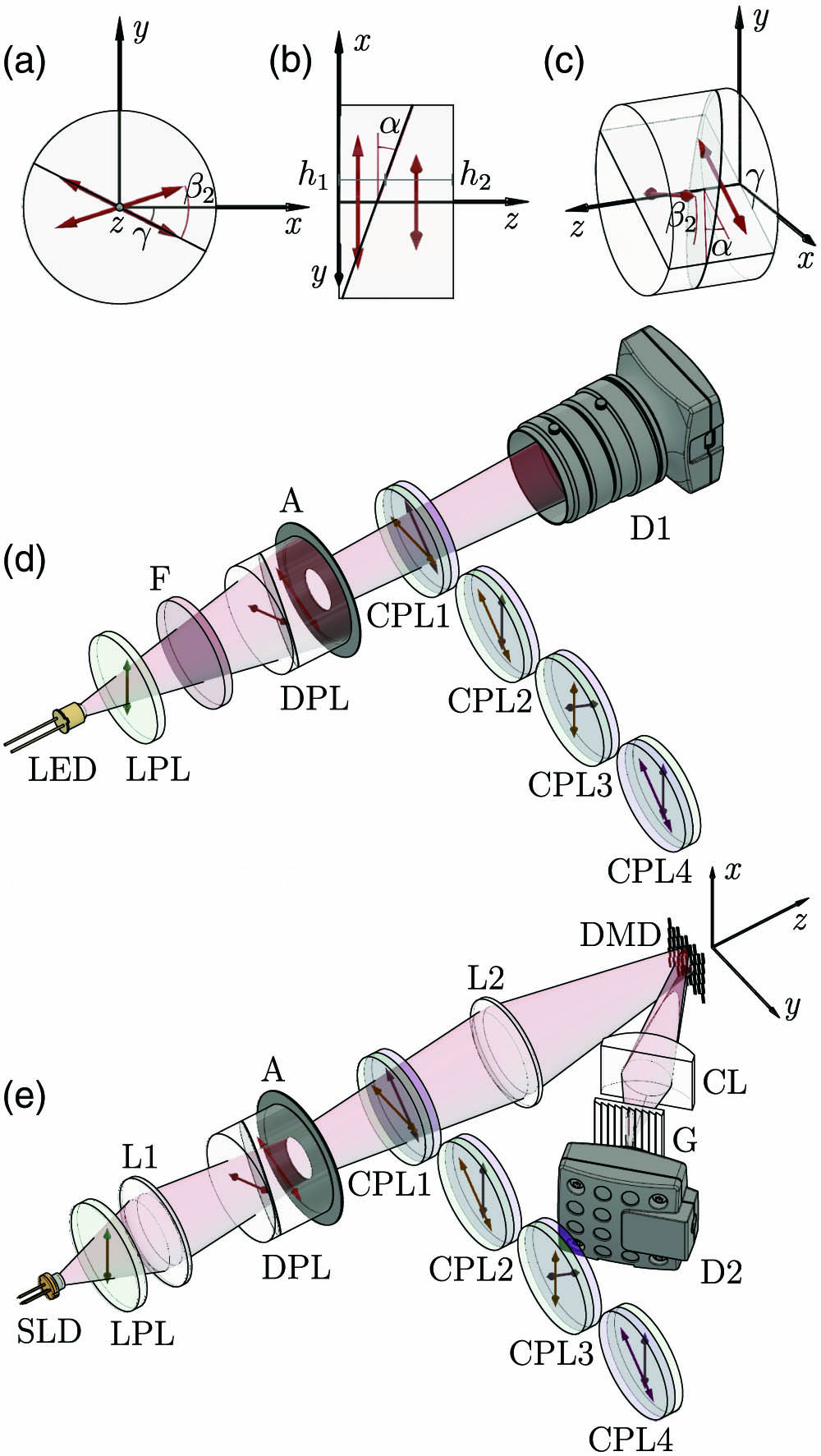
We modify the polarization properties of the SLD light with a quartz-wedge DPL (Thorlabs DPU-25-B), a deterministic element that can convert spectrally and temporally fully polarized light into a beam that is unpolarized in the time domain. This device consists of two birefringent quartz wedges (wedge angle α) with their optic axes rotated at β2=45° with respect to each other, as shown in Fig. 1(a). The Jones matrix of the DPL and its effect on the modes in Eq. (9) are analyzed in Appendix A. Since the retardation varies with position, an input beam that is uniformly fully polarized at a certain wavelength would produce an output beam with spatially periodic polarization modulation at that wavelength. As the retardation also varies with wavelength, the polarization-modulation fringes experience a lateral spectral shift. Hence, though the output beam is fully (but nonuniformly) polarized at each wavelength, the time-domain degree of polarization is less than unity. For sufficiently broadband incident light, the output appears highly unpolarized in the time domain.

These properties are more explicitly seen by considering the connection between the time-domain and frequency-domain polarizations ^[12,16,17]. The electromagnetic version of the Wiener–Khintchine theorem implies that where J(r) and ϕ(r,ω)=W(r,r,ω) are the time-domain and frequency-domain polarization matrices, respectively. For convenience, we expressed the spectral dependence via angular frequency ω instead of wavelength λ. Therefore, if ϕ(r,ω) of a broadband light experiences significant spectral variations, the integrated matrix, i.e., the time-domain polarization matrix, may feature a highly unpolarized field with J(r) proportional to nearly a unit matrix.

As a useful discussion prior to considering the electromagnetic coherence (or two-point) properties of the source, we analyze the pure polarization effects induced by the DPL. We characterized the polarization modulation of the DPL by measuring the conventional polarization (one-point) Stokes parameters using the setup depicted in Fig. 1(d). Light from an LED (Thorlabs LED635L with center wavelength 635 nm and spectral FWHM of about 15 nm) first passes through a linear polarizer (LPL), an interchangeable narrowband spectral filter, the DPL, and a 10 mm diameter aperture. Four circular polarizers (CPLs) (to be described in detail in Section 4) were used to measure the spatial distributions of the four polarization Stokes parameters of the beam exiting the aperture.

Figure 2 shows the effect of the DPL for different spectral widths of the incident light. Here the gray-scale background illustrates the first Stokes parameter S0(x,y), i.e., the intensity of light, which is almost uniform. The state of polarization is represented by means of polarization ellipses: the size of the ellipses visualizes the degree of polarization, while red and blue colors indicate right-hand and left-hand polarization, respectively. In Fig. 2(a), no spectral filter was applied, whereas filters with FWHM passbands of 10, 3, and 1 nm were used in Figs. 2(b), 2(c), and 2(d), respectively. Clearly, for the unfiltered LED light, the spectrally integrated output is nearly unpolarized. When the spectrum gets narrower, the degree of polarization increases, and clear polarization fringes become visible, as expected. The changes in the degree of polarization reveal that the spectral polarization state varies with wavelength on the nanometer scale.

To measure the coherence Stokes parameters, we use Young’s double pinhole interferometer based on a DMD (Texas Instruments DLP3000 with mirror spacing 10.8 μm) ^[11] equipped with a spectrometer grating and four CPLs ^[9]. The entire setup is illustrated in Fig. 1(e). An objective L1 (focal length F1=8mm) first collimates the light from the SLD on the DPL plane. Before the DPL there is an LPL to make sure the input light is uniformly linearly polarized. A 3 mm diameter aperture A placed immediately after the DPL limits the beam diameter. Because of the relatively small size of the DMD array, we demagnify the beam onto the plane of the DMD with a lens (L2) (focal length F2=75mm).

We measure the spatial coherence as a function of x1 and x2 by scanning the DMD mirrors along the x axis across the image of the DPL. The active DMD mirrors are tilted to reflect light towards the camera detector, as visualized in Fig. 1(e). Light from the active mirrors creates the desired interference pattern on the camera detector, while the rest of the light is mainly reflected into the opposite direction by the inactive mirrors. Spectral resolution is achieved by including a transmission-type diffraction grating G (period 3333 nm) and a cylindrical lens (CL) (focal length 40 mm, with focusing power in the y direction) in the setup. This arrangement provides a spectral resolution of 53.3 nm/mm, or 0.28 nm per camera pixel.

To measure the coherence Stokes parameters, we use four polarization-modulating elements (CPL1–CPL4) in front of the interferometric setup and repeat the coherence measurement for a beam passing through each of these elements in sequence. We use four commercially available CPLs, which consist of glued-together combinations of an LPL and a quarter-wave plate. In CPL1, CPL2, and CPL3, the polarizer faces the source, and the directions of the polarization axes are (nominally) 0°, 45°, and 90° with respect to the x axis. In these cases, the purpose of the wave plate is simply to compensate intensity losses in the fourth element, CPL4, where the wave plate faces the source and acts as a functional quarter-wave retarder. This collection of four elements allows the determination of the coherence Stokes parameters, as explained in the following section. However, some technical notes regarding the system may be appropriate at this point.

We could have employed only one LPL and one quarter-wave plate and rotated them into suitable orientations, but this would have required two high-precision computer-controlled rotation stages. Also, reflections between the two separated surfaces could have caused unwanted interference patterns, which now were avoided as the elements were cemented together. Therefore, it was simpler to use four separate (and low-cost) retarder/polarization components on a sliding sledge. In such a setting, precise positioning of these components is not an essential concern.

To ensure the repeatability of our results by other interested parties, we proceed to describe some details on extracting the polarization and coherence information from intensity data collected by the camera detector.

If the CPL elements are oriented ideally and their retardation is exactly δ=π/2, one can calculate the Stokes parameters from the intensities Ii(r), i∈{1,…,4}, on the camera transmitted through elements CPL i as ^[18] Here we have labeled the detected intensities (spectral densities) with the letter I to avoid confusion with other Stokes parameters. However, the components are not exactly ideal. In analyzing the results, we accounted for their precise properties by measuring their orientation and retardation errors. Then, instead of applying Eqs. (13)–(16), we employed somewhat lengthier recovery expressions, presented in Appendix B.

We assume that the detection area is in the paraxial domain near the (folded) optic axis in Fig. 1(e). Denoting the coordinate on the detector by x′, we set its origin at the center of the pinholes at x1 and x2. The electromagnetic interference law then states that when the light fields originating from the two pinholes propagate, the resulting Stokes-parameter interference fringes in the detector plane have the forms ^[3,6] where Sn(j)(x′,λ), j∈{1,2}, are the distributions observed when only the pinhole at position xj is open, and n∈{0,…,3}. Further, ϕn(x1,x2,λ)=arg[μn(x1,x2,λ)] and A(λ)=2πa/dλ, where a is the separation of the pinholes and d is the distance from the pinhole plane to the detector plane.

We extract the polarization fringes on the camera as so that with n∈{0,…,3}. The parameters Cn(x′,λ) then have real values in the range [−1,1]. We fit the cosine curves in Eq. (19) on the experimentally detected distributions in Eq. (18) to find the absolute values of μn(x1,x2,λ) from the amplitudes of the cosine curves and the spectral phases ϕn(x1,x2,λ) from the lateral positions of the fringes.

Clear visualization of three-dimensional coherence data contained in Sn(x1,x2,λ), n∈{0,…,3}, is somewhat challenging, and therefore we present different cross sections of them. Figures 3 and 4 depict examples of measured spectral polarization interference fringes corresponding to a single pinhole-coordinate pair (x1,x2)=(97.2μm,−97.2μm). The horizontal axis corresponds to the x′ coordinate on the detector, while the vertical axis represents the wavelength. Figure 3 displays the measurement results without the DPL, while Fig. 4 shows the results when the DPL is in place. In both figures, the left column illustrates the directly observed fringes Ii(x′,λ) when light is transmitted through the polarization elements CPL i, whereas the right columns show the fringes of Cn(x′,λ), calculated with Eqs. (B1)–(B4) and Eq. (18).

In Fig. 3, where the DPL is removed, the polarization state does not change with wavelength. Therefore, there is no spectral modulation in the fringe patterns, except that they appear slightly tilted because the fringe period increases with wavelength. Close to the optic axis (x′=0), no tilting takes place while the tilt increases with larger x′. The visibility of the fringes stays constant (within experimental errors) and the phases of the coherence Stokes parameters do not change with wavelength. In Fig. 4, where the DPL is present, the spectral polarization-coherence modulation is obvious. The fringe contrast and therefore the absolute values of |μn| vary as a function of λ, as do the positions of the fringes and thereby the phases arg(μn).

Figure 5 compares the simulated and measured quantities characterizing spatial coherence at a single wavelength. Figures 5(a), 5(c), 5(e), 5(g), and 5(i) depict the simulated values of μ0, μ1, μ2, μ3, and the electromagnetic degree of coherence μ, respectively. The corresponding measured data are shown in Figs. 5(b), 5(d), 5(f), 5(h), and 5(j). Figure 5(k) shows the measured spectrum of the light source and the vertical line indicates the wavelength λ=657.9nm at which the results are illustrated; a scan across the entire spectrum is shown in the Visualization 1. Since the coherence data are complex-valued, we illustrate the phase by color hue and the absolute value by brightness, as clarified in the two-axis color map in Fig. 5(l).

The match between the simulated and measured data is seen to be quite good. The electromagnetic degree of coherence μ(x1,x2,λ) is real-valued and rather featureless, as expected, since it should not change when unitary transformations such as wave plates (in the DPL) are applied to the light field. Therefore, the detected μ at any single wavelength with the DPL present should be identical to that of the input beam at the same optical path length. Small variations in the detected μ are visible, which are probably caused by imperfect calibration of the polarization measurement elements. The parameters used in the simulations are h¯1=2.47mm, h¯2=4.93mm, α=2°, β1=0°, β2=45°, γ=−37°, nf=1.5418, ns=1.5506 ^[19].

Figure 6 displays diagonal cross sections of the simulated coherence data cubes, evaluated at x1=x and x2=−x. The left column shows the spectral variation of |Sn(x,−x,λ)|, where the spectral and spatial intensity widths are visible. In the center column, the varying intensity is normalized out, leaving |μn(x,−x,λ)|. The right column depicts the phases arg[μn(x,−x,λ)]. We observe that the coherence Stokes parameters are quasi-periodic along both the spatial and spectral axes. Figure 7 illustrates the corresponding measurement data. The match is rather good; even the checkerboard-like pattern of the phase is somewhat visible. In general, Figs. 6 and 7 demonstrate that the spectral spatial coherence may vary with wavelength at the scale comparable to or less than a nanometer.

In the simulations we assumed that the detection plane is at the beam waist, and therefore all phase features are caused by the DPL modulation. In the measurement system, the lenses caused a spherical phase front and more complex aberrations in the detected field. To see the DPL effects alone, we removed these phase aberrations by measuring the phases of Sn(x1,x2,λ) for all n∈{0,…,3} without the DPL and by subtracting them from the phases of the data measured with the DPL.

We have demonstrated an experimental system for measuring the spectral coherence Stokes parameters using spectrally resolved Young’s interference fringes. It is a general-purpose measurement device not limited to the light source considered in this paper. The system can be used to characterize complicated spatio-spectral polarization and the coherence structure of lasers, LEDs, and other sources at visible optical frequencies, and can be modified to operate in other spectral regions as well. Information on the source coherence is of particular importance in analyzing the behavior of light in various optical systems.

The system has certain limitations, though many of them can be overcome. It can only measure spatial coherence on a line parallel to the x axis due to the fixed orientation of the CL and the spectrometer grating. Naturally, we could measure spatial coherence at other coordinate orientations by simply rotating the source about the z axis. The measurement speed might also be an issue, as every (x1,x2) pair is scanned separately. One possible way to increase the speed could be using several pinholes at a time instead of just two ^[20], though this would make the interpretation of the results more complicated and could reduce the signal-to-noise ratio. Also, the intensity of the input beam cannot be too low, as light is reflected from two micromirrors only, and thereafter spread into a spectrum.

One possible option (presently under investigation) to increase both the measurement speed and the light efficiency is to use wavefront folding and/or shearing interferometers ^[21] together with polarization measurement elements CPL1–CPL4. In all cases, one should make sure that the interferometer does not change the input polarization state, as this could lead to unwanted reduction of the fringe visibility and thus alter the measurement results.

We may also remark about using different light sources in the demonstrations of the polarization and spatial coherence measurements. For the former case, spectral filters and an LED source all operating at 635 nm were readily available. However, the spatial coherence width of the LED was too narrow for the coherence measurement, for which a more coherent wide-spectrum SLD source (centered at 670 nm) was employed. Even though we considered light beams with these particular wavelengths, the technique is generally valid over the whole visible bandwidth.

We characterized the coherence/polarization properties of a partially spatially coherent, nonuniformly polarized, secondary source of the type considered in Ref. ^[13], which, in addition, has a spectral width that prevents its description as a quasi-monochromatic source. We considered only the secondary source itself, but the system could equally be used to study experimentally the rich propagation phenomena predicted in Ref. ^[13]. To this end, one would need to use a spectral filter (as was done in Section 3) to narrow down the bandwidth of the field and then translate the entire measurement system in the direction of the beam propagation axis in order to image the transverse plane of interest onto the camera.

In this work, we introduced a simple and robust technique to measure the spatial and spectral distributions of the frequency-domain coherence Stokes parameters. The method is based on a DMD and a diffraction grating, and its validity was demonstrated by using a quartz-wedge DPL to prepare a beam with a complicated spatio-spectral coherence structure. Our results also show that the polarization and electromagnetic coherence properties may vary with wavelength on a scale less than a nanometer. The technique introduced in this work is of particular importance in analyzing the coherence-induced optical effects in various optical systems.

References

[1] L. Mandel, E. Wolf. Optical Coherence and Quantum Optics(1995).
Henri Partanen, Ari T. Friberg, Tero Set?l?, Jari Turunen. Spectral measurement of coherence Stokes parameters of random broadband light beams[J]. Photonics Research, 2019, 7(6): 669