Compensation of turbulence-induced wavefront aberration with convolutional neural networks for FSO systems

Min’an Chen; Xianqing Jin; Shangbin Li; Zhengyuan Xu

doi:10.3788/COL202119.110601

Abstract

To reduce the atmospheric turbulence-induced power loss, an AlexNet-based convolutional neural network (CNN) for wavefront aberration compensation is experimentally investigated for free-space optical (FSO) communication systems with standard single mode fiber-pigtailed photodiodes. The wavefront aberration is statistically constructed to mimic the received light beams with the Zernike mode-based theory for the Kolmogorov turbulence. By analyzing impacts of CNN structures, quantization resolution/noise, and mode count on the power penalty, the AlexNet-based CNN with 8 bit resolution is identified for experimental study. Experimental results indicate that the average power penalty decreases to 1.8 dB from 12.4 dB in the strong turbulence.

Keywords

free-space optical communication optical fiber wavefront aberration

1. Introduction

In practical outdoor free-space optical (FSO) communication systems, wavefront aberration is usually observed due to the atmospheric turbulence that causes random fluctuations in the air’s refractive index^[1–3]. At a lens-based optical receiver, extra loss is induced by low coupling efficiency of the aberrated light beam, which is coupled into a standard single mode fiber (SMF) followed by an optical detector/amplifier. To reduce the turbulence-induced power loss, the traditional adaptive optics (AO) is applied to compensate the wavefront aberration^[4–6], and this normally requires a wavefront sensor (WFS) for detection of the wavefront aberration. However, wavefront measurement becomes a challenge in the strong turbulence, as the method requires many sensing and control channels in the WFS for an aperture larger than the Fried parameter^[7].

To address this challenge, the WFS-less AO was investigated with blind optimization algorithms including simulated annealing (SA) and stochastic parallel gradient descent (SPGD)^[6–8]. In such WFS-less AO systems, the wavefront aberration is compensated iteratively to obtain a target performance metric, which is related to the laser beam quality, such as the far-field intensity distribution^[6]. Thousands of iterations and performance metric calculations are usually needed for converged performance.

As an emerging technology, deep learning has been recently studied for wavefront sensing/compensation in biomedicine, astronomy, and FSO systems with Gaussian or vortex beams^[9–16]. A WFS may not be required, as deep learning was applied to estimate the wavefront aberration directly from intensity images captured by a camera^{[11–13,15,16]}. These deep learning-based solutions include the convolutional neural network (CNN)^[11–13], back propagation (BP) artificial neural network^[15], and reinforcement learning with the Markov decision process^[16]. The CNN was applied on a point-spread function to achieve a good preliminary estimate, which improved the convergence performance (rate)^[10]. For the FSO applications, an optical feedback network making use of a CNN and a gradient descent optimizer was designed to mitigate the turbulence effect by adjusting the optical mode profiles at the transmitter^[17]. However, such a solution may confront the challenge of large latency in BP and image processing. In the above literature, most investigations were made by simulation irrespective of the practical components’ limitations, including image quality and coupling efficiency.

Sign up for Chinese Optics Letters TOC. Get the latest issue of Chinese Optics Letters delivered right to you！Sign up now

We experimentally demonstrated a solution of wavefront compensation with an AlexNet-based CNN without discussions about key limitation factors in FSO systems^[18]. To further study the effectiveness of the CNN-based solution for FSO system, in this Letter, an extended investigation is made on the impact of practical limitation factors on the aberration compensation performance. These factors include quantization resolution or noise of received intensity images, the number of Zernike modes (polynomials), and structure of the CNN. We construct the wavefront aberrations in a statistical way such that the light beams at the receiver can be modeled with Zernike modes in the Kolmogorov turbulence. To evaluate the CNN-based solution, the power penalty of the received light beam coupled into an SMF is studied in experiment.

2. Principle

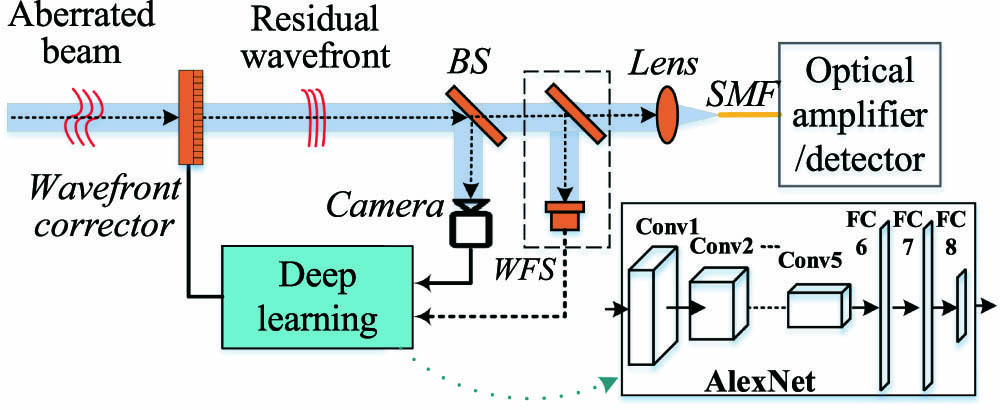
Figure 1 depicts a block diagram of an AO system with deep learning for FSO communication. There is atmospheric turbulence-induced wavefront aberration for the received light beam $ϕ (ρ, θ)$ . $ρ$ and $θ$ are the normalized polar radius and angle, respectively. Without compensation of the wavefront aberration, the aberrated light beam after the lens may not be efficiently coupled into an SMF-pigtailed optical detector (photodiode) or amplifier, thus causing a large power penalty/loss. Therefore, a wavefront corrector is applied to compensate the wavefront aberration estimated by the deep learning solution at the receiver. Residual wavefront may exist after the aberration compensation due to inaccurate estimation of the aberration. With beam splitters (BSs), a fraction of the light beam is captured by a camera, whilst the remainder of the light beam is coupled into an optical fiber of the optical detector. At the initial stage of the FSO link establishment, a deep learning network is trained with intensity images and phase, which are detected by the camera and WFS, respectively. After network training, the WFS may not be necessary, so only the camera is required.

Figure 1.Block diagram of an AO system with deep learning for FSO communication. BS, beam splitter. Inset: AlexNet structure.

The wavefront aberration is usually modeled with Zernike modes/polynomials in the atmospheric turbulence based on the Kolmogorov theory^[19,20]. Orthogonal Zernike modes/polynomials are used to form an aberrated wavefront, $ϕ$ : $ϕ (ρ, θ) = \sum_{k = 1}^{K} a_{k} Z_{k} (ρ, θ),$ (1) $Z_{k} = {\begin{cases} \sqrt{2 (n + 1)} R_{n}^{m} (ρ) \cos m θ, & m \neq 0, & k is even, \\ \sqrt{2 (n + 1)} R_{n}^{m} (ρ) \sin m θ, & m \neq 0, & k is odd, \\ \sqrt{(n + 1)} R_{n}^{0} (ρ), & m = 0 & , \end{cases}$ (2) $R_{n}^{m} (ρ) = \sum_{s = 0}^{(n - m) / 2} \frac{{(- 1)}^{s} (n - s)! ρ^{n - 2 s}}{s! [(n + m) / 2 - s]! [(n - m) / 2 - s]!},$ (3)where $a_{k}$ is the $k$ th Zernike mode coefficient. $m$ and $n$ are integers ( $m \leq n$ , $n - | m | = even$ ). $K$ is the number of modes. The Zernike coefficients are normally treated as zero-mean Gaussian random variables. However, the Zernike coefficients are not independent. To statistically model the atmospheric turbulence with correlated random variables, the covariance between coefficients $a_{i}$ and $a_{j}$ can be written as below^[21]: $E (a_{i}, a_{j}) = \frac{2.2698 \cdot {(- 1)}^{(n + n^{'} - 2 m) / 2} δ_{m m^{'}}}{Γ [(n - n^{'} + 17 / 3) / 2]} \cdot {(\frac{D}{r_{0}})}^{5 / 3} \cdot \frac{\sqrt{(n + 1) (n^{'} + 1)} \cdot Γ [(n + n^{'} - 5 / 3) / 2]}{Γ [(n^{'} - n + 17 / 3) / 2] \cdot Γ [(n + n^{'} + 23 / 3) / 2]},$ (4) $δ_{m m^{'}} = (m = m^{'}) \land [parity (i, j) \lor (m = 0)],$ (5)where $m$ ( $m^{'}$ ) and $n$ ( $n^{'}$ ) denote the azimuthal degrees and radial frequencies of $Z_{i}$ ( $Z_{j}$ ), respectively. $δ_{m m^{'}}$ is a logical Kronecker symbol. $Γ (\cdot)$ is a gamma function. $D / r_{0}$ represents atmospheric turbulence strength. $D$ is receiver aperture diameter, and $r_{0}$ denotes atmospheric coherent length. parity $(i, j)$ is one if the same parity occurs for indices $i$ and $j$ , otherwise, it is zero. The ‘ $\land$ ’ and ‘ $\lor$ ’ are logical operators of ‘and’ and ‘or’, respectively. The singular value decomposition (SVD) of the covariance matrix from Eq. (4) is applied to calculate a unitary matrix and a diagonal matrix for the independent Gaussian random variables generation. As a result, a random atmospheric wavefront is generated.

By applying the CNN, the aforementioned wavefront aberration can be estimated with intensity images of the received light beam, ${| F {E_{r} \exp [j ϕ (ρ, θ)]} |}^{2}$ . $E_{r}$ is the electric field of the arriving beam. $F (\cdot)$ represents two-dimensional Fourier transform. A typical CNN with a structure of AlexNet in Refs. [22,23] is applied in Fig. 1. There are eight layers in the AlexNet structure, including the first five convolutional layers and the last three fully connected layers. The role of the convolutional layers is to extract features of the input images. The output of the convolution operation is connected to the activation functions (rectified linear unit) for the final output feature map. The task of the AlexNet-based CNN is to search the mapping between Zernike coefficients vector $A = [a_{1}, a_{2}, \dots, a_{K}]$ and intensity images. In order to accurately estimate the wavefront aberration, a number of images and the corresponding Zernike coefficients are used to train the CNN. In the training stage, the network weights of the CNN are updated by the Adam algorithm for the gradient-based stochastic optimization [10]. The loss function is written as $L_{C} = E (| A - A_{e} |)$ . $E (\cdot)$ stands for expectation, and $A_{e}$ means the estimated Zernike coefficients vector.

3. Impacts of Zernike Modes, Quantization Noise, and CNN Structures

To evaluate key factors affecting the aberration compensation performance, investigations are made on the impacts of the number of Zernike modes, quantization resolution (noise) of images, and CNN structure on power penalty in the simulation. As the first three modes ( $Z_{1} - Z_{3}$ ) can be easily corrected, Zernike modes ( $Z_{4} - Z_{K}$ ) are used to simulate the turbulence-induced wavefront aberration^[24,25]. During the training stage, the turbulence strength ( $D / r_{0}$ ) is 0–16 for the mixed weak/strong turbulence. The power penalty is defined as the optical power difference measured at the optical fiber’s end with and without the turbulence. The number of estimated Zernike vectors is 50 for statistical study of the power penalty. These parameter values are set by default unless specified explicitly. As shown in Figs. 2(a) and 2(b), the power distribution is plotted as a function of the number of Zernike modes. Even though the first three modes are not considered, the first 10 and 21 modes account for 85.15% and 93.40% of the total energy, respectively. The main energy is distributed on the low-order modes. The power starts to converge towards one for $K > 10$ .

Figure 2.(a) Normalized power as a function of mode count and (b) phases of the first ten Zernike modes. Test error and power penalty for different (c), (d) numbers of Zernike modes (K), (e), (f) quantization bits, and (g), (h) CNN structures. (c)–(f) D/r₀ = 16. (g), (h) D/r₀ = 0–16.

The wavefront compensation performance with different numbers of Zernike modes is analyzed in the strong turbulence ( $D / r_{0} = 16$ ). To analyze the CNN-based estimation performance for different mode counts, the number of Zernike modes estimated with CNN is no larger than 45 randomly generated Zernike modes. It is seen from Figs. 2(c) and 2(d) that the test error with the AlexNet-based CNN increases with the number of Zernike modes. The average power penalty for $K = 10$ is slightly higher than that for $K = 45$ . This indicates that the test error may not be able to directly represent the wavefront compensation performance. The power penalty is essential to indicate power loss/efficiency at the receiver, which is the focus of this study. In addition, Fig. 2(d) shows a small variation in mean and standard deviation of power penalty estimated with the CNN even when some Zernike modes are not estimated. Such small variation is because of a majority of the power on the low-order modes. This reveals that a small number of Zernike modes can be used for the low-complexity purpose. Therefore, $K$ is set to 10 in the following study.

The impact of quantization bits on the wavefront compensation performance with the CNN is presented in Figs. 2(e) and 2(f) when $D / r_{0} = 16$ . The trends of the varied test error in the CNN for different quantization resolutions are almost the same. The average power penalty slightly decreases with increasing quantization bits. The variance in the power penalty for 4 bit resolution is slightly larger than that for 8/12/16 bit resolutions, which have almost the same performance. This is because the CNN has an advantage of combating quantization noise with a large amount of input data. Therefore, the optimum number of quantization bits of eight is suggested.

The CNN structure varies for different applications. We analyzed three different network structures: 4-layer LeNet, 8-layer AlexNet, and 19-layer VGG19. It is shown in Figs. 2(g) and 2(h) that AlexNet and VGG19 significantly reduce the power penalty for a number of Zernike modes up to 45 in the mixed weak/strong turbulence case ( $D / r_{0} = 0 - 16$ ). The average and deviation of power penalty increase with the number of Zernike modes, whilst the difference between AlexNet and VGG19 is very small. Before the CNN processing, the average and deviation remain relatively high. It is noted that for a large number of Zernike modes the simple structure of LeNet fails to estimate the wavefront aberration, which causes a large power penalty comparable to that before CNN. Considering the high complexity of VGG19, AlexNet with relatively low complexity has almost the same performance as VGG19. Therefore, the AlexNet-based CNN is chosen as a suitable solution in our experimental study.

Apart from the comparison among different CNN structures, traditional solutions of wavefront compensation (SPGD or SA)^[6–8] were utilized for performance comparison. As shown in Fig. 3, the power penalty with SPGD and SA sharply increases with the turbulence strength factor ( $D / r_{0}$ ). For the weak turbulence case when $D / r_{0} \leq 6$ , the power penalty with the AlexNet-based CNN is very close to that with SPGD/SA solutions. However, the difference in power penalty increases for large $D / r_{0}$ in the relatively strong turbulence case ( $D / r_{0} > 6$ ). This suggests that in the strong turbulence case the CNN outperforms the SPGD and SA. As there is no requirement of iterations, the CNN solution can be used to compensate wavefront aberration faster than the traditional solutions in the especially strong turbulence case after the CNN is trained.

Figure 3.Comparison in power penalty among SPGD, SA, and AlexNet-based CNN.

4. Experimental Results and Discussions

Figure 4 depicts an experimental setup of a CNN-based AO system and its corresponding block diagram for FSO applications. A standard fiber-pigtailed distributed feedback (DFB) laser operating at a wavelength of 1550 nm is used to emit a Gaussian beam. The DFB laser was connected to a collimator, half-wave plate, and polarizer such that vertically polarized transmission was realized as required by a phase-only spatial light modulator (SLM). The propagation beam diameter is 7 mm. Random phase patterns produced with Zernike modes were introduced by the SLM with a pixel count of $1920 \times 1080$ and a pixel pitch of 8.0 µm (Holoeye PLUTO-TELCO-013) in order to generate wavefront aberration for different atmospheric turbulence cases. The SLM can also be used for compensation of the wavefront aberration that is estimated with the CNN. A BS with a split ratio of 50:50 was utilized to split the received light into two beams, each of which reaches an infrared charge-coupled device (CCD) camera ( $640 \times 512$ pixels, Bobcat-640-GigE) or an SMF. The laser’s launch power was 11.8 dBm. The batch size is 16.

Figure 4.Experimental setup for evaluation of a CNN-based AO system and the corresponding block diagram.

For training the AlexNet-based CNN, 16,000 datasets of wavefront aberrations together with a number of epochs were produced with different atmospheric turbulence strength values. The intensity images corresponding to the wavefront aberrations were captured by the CCD camera. The training dataset consisting of wavefront aberrations and corresponding intensity images were sent to the CNN for the TensorFlow-based training. Another 2000 datasets were used to calculate test errors. Once the AlexNet-based CNN is trained, we can estimate the Zernike coefficients for the wavefront aberrations, the conjugation of which was used for the wavefront compensation at the SLM.

In order to evaluate the loss performance in the training stage, the curves of the loss versus epochs are shown in Fig. 5(a), where both experimental and numerical (simulation) results are presented for comparison. An epoch means one pass of a full training set. As seen in the figure, the simulated loss performance converges faster than experimentally measured loss. A minimum of 1 and 5 epochs are observed for converged performance in the simulation and experiment, respectively. This may be due to the background noise of the CCD camera with limited amount of pixels in the experiment.

Figure 5.(a) Loss performance versus epochs for training CNN. (b) Estimated Zernike coefficients and absolute errors. (c) Wavefront aberration and (d) corresponding intensity images (D/r₀ = 16).

As an example, a random Zernike coefficient vector is used for generation of a wavefront aberration ( $D / r_{0} = 16$ ) in Fig. 5(c). We observed a dispersed speckle in the camera, as shown in Fig. 5(d). In order to understand the experimental phenomenon, the CNN-based wavefront compensation was also numerically investigated for comparison in Fig. 5(b). The Zernike coefficients estimated in simulation and experiment are almost identical to the theoretical values. The calculated absolute errors of Zernike coefficients are smaller than 0.25. A circular speckle was thus observed after the wavefront compensation in Fig. 5(d).

The performance of the CNN-based wavefront compensation was further investigated statistically with 50 random Zernike vectors for different wavefront aberrations in experiment. The relatively weak or strong ( $D / r_{0} = 4$ or 16) turbulence cases were considered in Fig. 6, where the box plot of the measured power penalty denotes its range and mean. Thanks to the CNN-based wavefront compensation, the mean/variance (power penalty) significantly decreases. The mean of the power penalty reduces to 1.8 (0.8) dB from 12.4 (4.4) dB for $D / r_{0} = 16$ (4) in the strong (weak) turbulence. In the inset of the figure, the constellation of power penalty versus the root mean square (RMS) of wavefront errors is given to further understand the result. Although the constellation points are dispersed, the power penalty is nearly proportional to the RMS wavefront errors. However, the variance of the power penalty increases for large RMS. The dispersed constellation suggests that the performance of the CNN-based wavefront compensation may not be well indicated with the RMS for FSO applications. Given the difficulty in measuring wavefront aberrations, the optical power can be monitored as a simple way for indicating the wavefront compensation performance.

Figure 6.Power penalty in the weak/strong turbulence case. Inset: power penalty versus RMS of estimated wavefront errors (D/r₀ = 16).

5. Conclusions

An AlexNet-based CNN for the atmospheric turbulence-induced wavefront aberration compensation for FSO applications has been investigated in experiment and simulation. Statistically constructed wavefront aberrations were used for the aberrated light beams with the Zernike modes (polynomials) theory. To explore the effectiveness of the AlexNet-based CNN solution, we have analyzed three key factors affecting the compensation performance, which include CNN structures, Zernike mode count, and quantization resolution (noise) of intensity images. AlexNet was identified as an appropriate CNN structure by considering a trade-off between the power penalty and complexity. Experimental results indicate that the power penalty reduces to 1.8 dB from 12.4 dB for the strong turbulence case. As one of the key challenges for outdoor FSO applications, the background noise and/or inference will be studied in the future.

References

[1] H. Kaushal, G. Kaddoum. Optical communication in space: challenges and mitigation techniques. IEEE Comm. Surv. Tutor., 19, 57(2017).

[2] T. Shan, J. Ma, T. Wu, Z. Shen, P. Su. Single scattering turbulence model based on the division of effective scattering volume for ultraviolet communication. Chin. Opt. Lett., 18, 120602(2020).

[3] X. Yan, L. Guo, M. Cheng, S. Chai. Free-space propagation of autofocusing Airy vortex beams with controllable intensity gradients. Chin. Opt. Lett., 17, 040101(2019).

[4] C. Liu, M. Chen, S. Chen, H. Xian. Adaptive optics for the free-space coherent optical communications. Opt. Commun., 361, 21(2016).

[5] M. Li, W. Gao, M. Cvijetic. Slant-path coherent free space optical communications over the maritime and terrestrial atmospheres with the use of adaptive optics for beam wavefront correction. Appl. Opt., 56, 284(2017).

[6] Y. Liu, J. Ma, B. Li, J. Chu. Hill-climbing algorithm based on Zernike modes for wavefront sensorless adaptive optics. Opt. Eng., 52, 016601(2013).

[7] P. Piatrou, M. Roggemann. Beaconless stochastic parallel gradient descent laser beam control: numerical experiments. Appl. Opt., 46, 6831(2007).

[8] Z. Li, J. Cao, X. Zhao, W. Liu. Atmospheric compensation in free space optical communication with simulated annealing algorithm. Opt. Commun., 338, 11(2015).

[9] J. Liu, P. Wang, X. Zhang, Y. He, X. Zhou, H. Ye, Y. Li, S. Xu, S. Chen, D. Fan. Deep learning based atmospheric turbulence compensation for orbital angular momentum beam distortion and communication. Opt. Express, 27, 16671(2019).

[10] S. W. Paine, J. R. Fienup. Machine learning for improved image-based wavefront sensing. Opt. Lett., 43, 1235(2018).

[11] Y. Jin, Y. Zhang, L. Hu, H. Huang, Q. Xu, X. Zhu, L. Huang, Y. Zheng, H. Shen, W. Gong, K. Si. Machine learning guided rapid focusing with sensor-less aberration corrections. Opt. Express, 26, 30162(2018).

[12] Q. Tian, C. Lu, B. Liu, L. Zhu, X. Pan, Q. Zhang, L. Yang, F. Tian, X. Xin. DNN-based aberration correction in a wavefront sensorless adaptive optics system. Opt. Express, 27, 10765(2019).

[13] Y. Nishizaki, M. Valdivia, R. Horisaki, K. Kitaguchi, M. Saito, J. Tanida, E. Vera. Deep learning wavefront sensing. Opt. Express, 27, 240(2019).

[14] R. Swanson, M. Lamb, C. Correia, S. Sivanandam, K. Kutulakos. Wavefront reconstruction and prediction with convolutional neural networks. Proc. SPIE, 10703, 107031F(2018).

[15] Z. Li, X. Zhao. BP artificial neural network based wave front correction for sensor-less free space optics communication. Opt. Commun., 385, 219(2017).

[16] K. Hu, B. Xu, Z. Xu, L. Wen, P. Yang, S. Wang, L. Dong. Self-learning control for wavefront sensorless adaptive optics system through deep reinforcement learning. Optik, 178, 785(2019).

[17] S. Lohani, R. T. Glasser. Turbulence correction with artificial neural networks. Opt. Lett., 43, 2611(2018).

[18] M. Chen, X. Jin, Z. Xu. Investigation of convolution neural network-based wavefront correction for FSO systems. International Conference on Wireless Communication and Signal Processing, 1(2019).

[19] R. J. Noll. Zernike polynomials and atmosphereic turbulence. J. Opt. Soc. Am. A, 66, 207(1976).

[20] N. A. Roddier. Atmospheric wavefront simulation using Zernike polynomials. Opt. Eng., 29, 1174(1990).

[21] X. Yin, X. Chen, H. Chang, X. Cui, Y. Su, Y. Guo, Y. Wang, X. Xin. Experimental study of atmospheric turbulence detection using an orbital angular momentum beam via a convolutional neural network. IEEE Access, 7, 184235(2019).

[22] S. B. Driss, M. Soua, R. Kachouri, M. Akil. A comparison study between MLP and convolutional neural network models for character recognition. Proc. SPIE, 10223, 1022306(2017).

[23] A. Krizhevsky, I. Sutskever, G. E. Hinton. ImageNet classification with deep convolutional neural networks. Advances in Neural Information Processing Systems, 1097(2012).

[24] D. G. Sandler, T. K. Barrett, D. A. Palmer, R. Q. Fugate, W. J. Wild. Use of a neural network to control an adaptive optics system for an astronomical telescope. Nature, 351, 300(1991).

[25] G. Xu, X. Zhang, J. Wei, X. Fu. Influence of atmospheric turbulence on FSO link performance. Proc. SPIE, 5281, 816(2004).