An Improved Single-Frame Super-Resolution Algorithm for Magnetic Resonance Image

Jinghui Chu; Fengshuo Hu; Jiaqi Zhang; Wei Lü

doi:10.3788/LOP55.051009

Journals >Laser & Optoelectronics Progress >Volume 55 >Issue 5 >Page 051009 > Article

Laser & Optoelectronics Progress
Vol. 55, Issue 5, 051009 (2018)

An Improved Single-Frame Super-Resolution Algorithm for Magnetic Resonance Image

Jinghui Chu, Fengshuo Hu, Jiaqi Zhang, and Wei Lü^*;

Author Affiliations

School of Electrical and Information Engineering, Tianjin University, Tianjin 300072, China

show less

DOI: 10.3788/LOP55.051009 Cite this Article Set citation alerts

Jinghui Chu, Fengshuo Hu, Jiaqi Zhang, Wei Lü. An Improved Single-Frame Super-Resolution Algorithm for Magnetic Resonance Image[J]. Laser & Optoelectronics Progress, 2018, 55(5): 051009 Copy Citation Text

show less

An example of stationary wavelet transform using db2 in internal dataset. (a) Original image; (b)-(d) horizontal, vertical, diagonal high frequency of 1-level SWT; (e)-(g) horizontal, vertical, diagonal high frequency of 2-level SWT

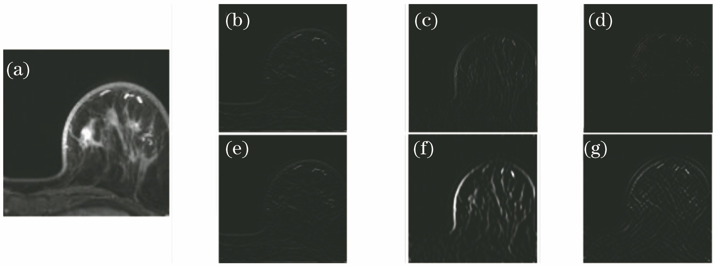
Fig. 1. An example of stationary wavelet transform using db2 in internal dataset. (a) Original image; (b)-(d) horizontal, vertical, diagonal high frequency of 1-level SWT; (e)-(g) horizontal, vertical, diagonal high frequency of 2-level SWT

Download full size

Fig. 2. Demonstration of overlapping separating

Download full size

Fig. 3. Framework of proposed super-resolution method

Download full size

Fig. 4. Visual comparison of 3×upscaling reconstruction effect. (a) Original image; (b) bicubic interpolation; (c) method in Ref. [5]; (d) method in Ref. [6]; (e) SRCNN; (f) proposed method (with haar)

Download full size

Window size /(pixel×pixel)	PSNR	SSIM	RLNE	EPI
2×2	28.4266	0.9939	0.0232	1.3792
3×3	28.5170	0.9941	0.0228	1.3618
5×5	28.3959	0.9935	0.0234	1.3691
7×7	28.2219	0.9933	0.0239	1.3858

Table 1. Comparison of different patch sizes (3×upscaling, dictionary size 500, clustering number 3, wavelet base db2)

Dictionarysize	PSNR	SSIM	RLNE	EPI
2000	28.6238	0.9945	0.0222	1.4045
1000	28.6330	0.9945	0.0222	1.3779
500	28.5170	0.9941	0.0228	1.3618
100	28.2422	0.9928	0.0242	1.3657

Table 2. Comparison of different dictionary sizes (3×upscaling, patch size 3 pixel×3 pixel, clustering number 3, wavelet base db2)

Clusteringnumber	PSNR	SSIM	RLNE	EPI
3	28.6330	0.9945	0.0222	1.3779
4	28.5408	0.9941	0.0226	1.3657
5	28.5996	0.9943	0.0223	1.3807

Table 3. Comparison of different clustering numbers (3×upscaling, patch size 3 pixel×3 pixel, dictionary size 1000, wavelet base db2)

Index	haar	db2	db3	db4	sym2	sym3	sym4	sym6	sym8	coif1	coif2	dmey
PSNR	28.7574	28.6330	28.5366	28.6411	28.5444	28.6124	28.5836	28.5155	28.4995	28.5814	28.603	28.3491
SSIM	0.9949	0.9945	0.9941	0.9943	0.9941	0.9943	0.9945	0.9942	0.9941	0.9945	0.9941	0.9938
RLNE	0.0215	0.0222	0.0227	0.0221	0.0226	0.0223	0.0224	0.0228	0.0228	0.0224	0.0223	0.0237
EPI	1.3583	1.3657	1.3728	1.3576	1.3690	1.3561	1.3675	1.3671	1.3777	1.3701	1.3575	1.3766

Table 4. Comparison of different wavelet bases (3×upscaling, patch size 3 pixel×3 pixel, dictionary size 1000, clustering number 3)

Algorithm	MRI				DCE-MRI
Algorithm	PSNR	SSIM	EPI	RLNE	PSNR	SSIM	EPI	RLNE
Bicubic interpolation	30.1714	0.8817	0.4475	0.0348	32.4535	0.8854	0.5003	0.0094
Ref. [5]	31.2093	0.8945	0.5570	0.0274	33.8091	0.8923	0.5718	0.0070
Ref. [6]	31.5505	0.9025	0.5641	0.0254	34.2530	0.9059	0.6290	0.0062
Ref. [7]	31.7256	0.8984	0.5820	0.0330	34.0285	0.8698	0.6237	0.0148
db2	31.7225	0.9040	0.5721	0.0244	34.3888	0.9066	0.6343	0.0060
haar	31.7220	0.9036	0.5740	0.0245	34.5002	0.9072	0.6343	0.0058
sym4	31.7052	0.9041	0.5705	0.0244	34.3643	0.9066	0.6356	0.0061
db2_IBP	31.8756	0.9089	0.6141	0.0238	34.6785	0.9135	0.6831	0.0056
haar_IBP	31.8918	0.9088	0.6147	0.0240	34.5985	0.9104	0.6897	0.0057
sym4_IBP	31.8480	0.9089	0.6155	0.0237	34.4396	0.9094	0.6897	0.0060

Table 5. Comparison of 3×upscaling reconstruction effect of different methodsdB

Jinghui Chu, Fengshuo Hu, Jiaqi Zhang, Wei Lü. An Improved Single-Frame Super-Resolution Algorithm for Magnetic Resonance Image[J]. Laser & Optoelectronics Progress, 2018, 55(5): 051009

Download Citation

Set citation alerts for the article

Tools

Set citation alerts for the article

Save the article for my favorites

Paper Information