As is well understood, the random distribution of light intensity formed in space after the coherent light wave is scattered by a rough surface or a random medium is called speckle^[1,2]. Generally speaking, the characteristics of speckle are determined by the rough surface, random medium (scatterer), and the optical system that the scattered light waves pass by. The influence of scattering distance on speckle is also very important, generally divided into far-field speckle and near-field speckle. The far-field speckle is further divided into the Fraunhofer diffraction region and the Fresnel diffraction region, both of which belong to Gaussian speckle. Near-field speckle is generally considered to be the light intensity distribution within one wavelength from the surface of the scatterer. This area contains rich sub-micron optical information that cannot be detected by conventional optical methods. The deep Fresnel region is generally understood to be between the far field and the near field, approximately distributed between one to dozens of wavelengths. The speckle in this area also contains a lot of information on the random surface^[3–5].

For deep Fresnel region speckle (DFRS), due to the extremely close distance between the random surface and the observation surface, when the scattered light propagates from the random surface to the observation surface, it may be blocked by the fluctuations of the adjacent micro-surface, resulting in some scattered light not being able to reach the observation surface. This phenomenon is called the shadowing effect^[6–8]. The influence range of the shadowing effect will be affected by the scattering distance and the surface roughness. Most early studies used optical scattering theory to directly calculate the contribution of each point on the random surface to the observation surface, and they calculated the speckle field using the principle of light wave superposition^[9–13] without considering the shadowing effect.

The recent study of shadowing effect is contributed by Sun et al.^[8]. He defined the three-dimensional (3D) attenuation factor on the real surface, derived four functions that affect the 3D attenuation factor and performed calculations, discussed the effects of masking on the illumination, and defined a boundary where the shadowing or masking occurs. However, these theories are only used to calculate the attenuation of reflection, and there is not a proper explanation for the shadowing effect of the scattering in the deep Fresnel region. In this paper, we firstly simulate the generation of a 3D self-affine fractal random surface h(x,y). We improve the method of Sun et al. by using the light scattering theory and Kirchhoff approximation^[14] to simulate DFRS at different scattering distances under the premise of considering the shadowing effect. Because the simulation considers the effect of all surfaces around the observation point on the shadowing effect, the simulation of DFRS is more accurate.

Our work makes the following contributions.(1)The speckle evolution within one wavelength from the highest point of the random surface is studied.(2)The relationship between speckle within one wavelength from the highest point of the random surface and the surface morphology is studied.(3)The probability distribution of speckle intensity is studied and compared with the experimental measurement results.

The height of the random surface is a function of position coordinates, denoted as h(x0,y0). We use the following Fourier transform as the expression for generating the complex height function hc(x0,y0):$$\begin{gathered} hc(x0,y0)=hr(x0,y0)+jhi(x0,y0) \\ =2∬−∞+∞p(x01,y01)η(x01,y01)⁢exp[−j2π(xx0+y01y0)]dx01dy01, \end{gathered}$$(1)p(x01,y01)=[P(x01,y01)]1/2,(2)P(x01,y01)=∬−∞+∞ω2exp{−[(x0+y0)/ξ]2α}⁢exp[j2π(x01x0+y01y0)]dx0dy0,(3)where p(x01,y01)^[15] represents the aperture function; ξ is the correlation length of the surface, which characterizes the horizontal and vertical correlation range of the random surface; ω denotes the mean square deviation roughness of the surface (roughness for short), which describes the oscillation amplitude of the surface height deviating from the average height of the surface; α(0<α≤1) is the fractal index of the surface, which describes the local roughness of the surface. The smaller the value of α, the rougher the local surface. hr(x0,y0) and hi(x0,y0) are the real and imaginary parts of hc(x0,y0), respectively, and η(x01,y01) is the real variable white noise process with a mean of zero. Due to the characteristics of the speckle field, we can see that both hr(x0,y0) and hi(x0,y0) are Gaussian random processes with an average value of zero; both hr(x0,y0) and hi(x0,y0) can be used as the numerical distribution function of the height of the self-affine fractal surface.

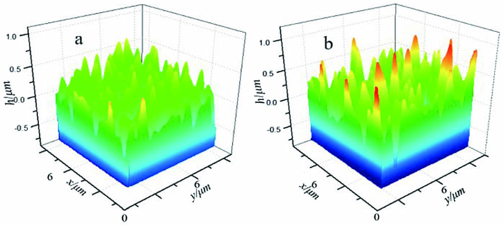
Figure 1 is the two surfaces we generated: Fig. 1(a) is a random surface with α of 1.0, ξ of 0.5 µm, and ω of 0.2 µm, and Fig. 1(b) is a random surface with α of 1.0, ξ of 0.5 µm, and ω of 0.3 µm. Each surface is generated from 1000×1000 data points with a spacing of 10 nm between points. It can be seen in Figs. 1(a) and 1(b) that the amplitude of the random surface with ω of 0.3 µm has a larger fluctuation range than the surface with ω of 0.2 µm, and there is no local small-scale fluctuation on both surfaces. In this paper, only the speckle properties of these two surfaces are discussed.

In order to understand the shadowing effect more intuitively, only the plane view is shown here. Figure 2 shows the process of light waves scattered by the random scattering surface propagating upward to the observation surface. Each scattered light leaving the surface is treated as a point light source for spherical wave propagation. After the light beam L1 scatters through the surface, it will begin to propagate in the form of a spherical wave from point N. Due to the blocking of the second peak to the left of point N and the first peak to the right, the light can only illuminate R-S area on the observation surface. In the meantime, the left side of the point R and the right side of the point S are blocked. Similarly, the light beam L2 can only illuminate the P-Q area after surface scattering. Due to the random fluctuation of the surface, it is impossible to solve the shadowing of different points with the unified standard. It can only be analyzed point by point.

It can be seen that whether the transmitted light can be completely blocked depends on whether it passes through the convex micro-surface on its propagation path. Because of this, we introduced two slope functions k1 and k2 in the simulation process. k1 is the slope of the line between the starting point of the transmitted light on the scattering surface and the possible observation point, and k2 is the maximum slope of the line between the starting point of the scattered light and the scattered surface point, which is from the starting point of the scattered light to the corresponding observation point. Obviously, when k1>k2, all of the points on the scattering surface are under the scattered light, so the scattered light will not be blocked. When k1≤k2, the scattered light will pass through the convex part of the scattering surface in a certain area, so the light is blocked from reaching the observation surface. Figure 3 shows the shadowing judgment process of scattered light, where E and F are two possible points of scattered light propagating from the point O (located on the random surface) to the observation surface. For point E, its corresponding k1=y1/x1, k2=y2/x2; because k1>k2, the light can propagate to point E. For point F, its corresponding k1=y3/x3, k2=y4/x4; because k1<k2, the light is blocked by the surface and cannot reach point F, which does not contribute to the light field at this point. In the calculation process, we do not consider the effect of secondary scattering or multiple scattering after the light is blocked. The scattering field calculated in this way is closer to the actual scattering process than without considering the shadowing effect. If it is used to calculate DFRS, the result should be more accurate than the traditional one without considering the shadowing effect. The calculation process of DFRS under the shadowing effect is discussed below.

The generation process of DFRS is shown in Fig. 4. A monochromatic incident beam with the amplitude of U0 and wavelength of λ illuminates perpendicularly on a random scattering surface placed on the object surface. The unit normal vector at any point on the scattering surface at A0(x0,y0) is represented by n⇀, and the height of the point is h(x0,y0) (shown in the enlarged section view). The distance between the observation surface A(x,y) located in the deep Fresnel region and the bottom of the scattering surface (at z=0) is z′. According to Kirchhoff’s approximation, the complex amplitude of the scattered light field at A(x,y) on the observation surface can be expressed as follows:U(x,y)=14π∬[G∂U0(x0,y0)∂n−U0(x0,y0)∂G∂n]dS0,(4)U0(x0,y0)=exp[jk(m−1)h(x0,y0)],(5)G=exp(jkr)r,(6)r={(x−x0)2+(y−y0)2+[z′−h(x0,y0)2]}1/2,(7)where G represents Green’s function, S0 is a random scattering surface, m is the refractive index of the medium on the random surface, k=2π/λ is the wave vector, and r is the distance between the scattering point and the field point A(x,y) on the random surface.

Because the normal derivative satisfies the following relationship:∂∂n=(n×∇)=1γ[−∂h(x0,y0)∂x0∂∂x0−∂h(x0,y0)∂y0∂∂y0+∂∂z],(8)γ={1+[∂h(x0,y0)∂x0]2+[∂h(x0,y0)∂y0]2}1/2,(9)therefore, Eq. (4) can be written as$$\begin{gathered} U(x,y)=14π∬dS0[G∂U0(x0,y0)∂n−U0(x0,y0)∂G∂n] \\ =14π∬dS0exp{jk[(m−1)h(x0,y0)+r]}⁢[jk(m−1)γr−(jk−1r)χr2], \end{gathered}$$(10)χ=h(x0,y0)−z′−(x0−x)∂h(x0,y0)∂x0−(y0−y)∂h(x0,y0)∂y0.(11)

If the shadowing effect is not considered, then Eq. (10) needs to integrate the entire scattering surface without judgment, which obviously does not conform to the actual scattering process. Therefore, before integration, we first determine whether the light is blocked according to the size of the two slopes k1 and k2, and only take the unblocked scattering points that satisfy k1>k2 for integration. If k1<k2, then we set the light wave contribution of the scattering point to zero directly. Obviously, the rougher the random surface and the closer the observation surface to the scattering surface, the greater the chance of the light wave being blocked.

Finally, we use the formula I(x,y)=U(x,y)·U*(x,y) to determine the light intensity distribution of the speckle field.

Based on the above theory, speckles between z=λ/10 and z=λ from the highest point of the random surfaces have been generated, with a wavelength of 632.8 nm. Considering the random surface height fluctuations, such as the roughness of 0.2 µm and 0.3 µm, the maximum height of the surface is 0.5678 µm and 1.0228 µm, respectively. Therefore, the distance between the observation surface and the scattering surface is completely located in the deep Fresnel region. Figure 5 shows some speckles generated at different z: for the first row of the scattering surface α=1, ξ=0.5µm, ω=0.2µm, for the second row of the corresponding scattering surface α=1, ξ=0.5µm, ω=0.3µm, and z gradually increases from left to right.

The evolutionary trend of the speckle with z changing in Fig. 5 can be clearly seen; when z is smaller, the speckle patterns are smaller, the distribution of bright spots is more uniform, and the speckle contrast is smaller. This is because the fluctuation of the surface is lower on the surface with less roughness, which makes the superposition of light waves insufficient. As a result, the bright spots in the speckle field are not too bright, the dark spots are not very dark, and the speckle contrast is relatively small. If the roughness is increased, the surface has a higher range of fluctuations, and different peaks and valleys have great differences in light scattering and shadowing effects. For example, high peaks and deep valleys are more helpful for scattering, resulting in some bright spots becoming brighter; some dark spots will also be darker, and their contrast is significantly increased. By using C=[(<I2>−<I>2)/<I>2]1/2 to calculate the contrast of speckle, we find that with the increase of the scattering distance, the speckle field alternates between light and dark spots, and the speckle contrast is gradually increased. For instance, when z gradually increases from λ/10 to λ, the speckle contrast of ω = 0.2 µm gradually increases from 0.9564 to 1.1601, reaching a maximum of 1.5598; while the speckle contrast of ω = 0.3 µm gradually increases from 1.1711 to 1.2484, the maximum reaches 1.4208. This is because the distribution of DFRS is strongly affected by surface fluctuations. If the peaks and valleys of the surface are regarded as micro convex lenses (Ls) and micro concave Ls^[16], respectively, there will not be bright spots that are too strong; when the roughness is small, and the distance between the observation surface and the scattering surface is less than the focus of these “Ls”, the speckle contrast is less than 1.0. As the distance increases to the value range of these foci, the intensity of some bright spots suddenly increases, resulting in the speckle contrast being greater than 1.0. The greater the number of “micro-Ls” whose foci are closer to the distance, the greater the contrast is. If the roughness is relatively large, and the surface has a greater fluctuation range, the minimum distance from the observation surface is roughly distributed within the focus of the “micro-L” on the surface, resulting in speckle contrasts greater than 1.0.

The light intensity probability density function is also one of the important parameters to describe speckle. For Gaussian speckle, it is a negative exponential function:PI(I)=1<I>exp(−I<I>),(12)where <I> is the average value of the speckle intensity. In order to facilitate the comparison between different speckle fields, the above formula is multiplied by <I> to become the normalized probability distribution function P(I), that isP(I)=exp(−I<I>).(13)

In the experiment, we used a microscopic imaging system (as shown in Fig. 6) to measure DFRS. The linearly polarized light generated by the He–Ne laser illuminates a random surface sample placed on a two-dimensional nano mobile platform (NMP) vertically, using a microscope objective (MO, 50×, numerical aperture of 0.75) and a focal length convex L (focal length of 12 cm) to enlarge the speckle field close to the random surface (ω=0.48µm, ξ=4.14µm, α=0.65). The enlarged image is recorded by a back-illuminated scientific complementary metal–oxide–semiconductor (s-CMOS) camera (Dhyana 400BSI V2.0, number of pixels 2048×2040, pixel size 6.5µm×6.5µm).

DFRS is more affected by the fluctuation of the scattering surface and is no longer Gaussian speckle. Figure 7 shows the normalized probability distribution of intensity about the Gaussian speckle, experimentally measured speckle, and DFRS, which is produced by a random surface with a roughness of 0.3 µm at different z values. It can be seen that the probability distribution of the intensity of DFRS is significantly different from the Gaussian speckle. The light intensity probability distribution of DFRS is lower than that of Gaussian speckle in the area with lower light intensity, and it increases significantly near the maximum light intensity. This is because, in the deep Fresnel region, scattering and superposition are insufficient, and there are very few points of fully destructive interference and destructive interference, so the area with light intensity close to zero is less than Gaussian speckle. Due to the “micro-L” effect of the fluctuation of the random surface, the Fresnel deep area observation surface may coincide with the focal plane of some “micro-Ls”, so varying amounts of light intensity of extremely strong points are generated. This results in a high light intensity area, and the probability distribution of DFRS is usually higher than that of Gaussian speckle. Of course, if the observation surface does not coincide with any focal plane, due to insufficient scattering and superposition, the probability of high light intensity is lower (as shown in the case of z=λ/10 in Fig. 7). It can be seen that the experimental curve in the area with a high light intensity is in good agreement with the simulation, while the area with a low-light intensity is obviously inconsistent with the simulation, and the probability increases. This may be due to the influence of camera noise, and some low-value noise signals will appear in the measurement of the speckle field. In addition, the numerical aperture of the MO also limits the range of the recorded light wave.

We also found that the probability distribution of DFRS intensity is also related to the surface roughness. Under the same z, the greater the surface roughness, the greater the proportion of bright spots is in the intensity probability distribution. This is because the greater the roughness of the surface and the greater the fluctuation of the surface, the greater the proportion of micro-Ls that form a smaller focal length, which causes more light to converge on the observation surface to form more extreme bright spots.

Since DFRS contains a lot of information on the random surface, we might as well explore the relationship between the morphology of the scattering surface and the speckle. As the distribution of speckle at different scattering distances is very different, after comparison, we found that at some specific distances the intensity distribution of DFRS is very similar to the morphology of its scattering surface, and the greater the roughness, the farther the specific scattering distance.

Figure 8 shows comparison between the scattering surface with different roughnesses (ω=0.2µm and ω=0.3µm) and the intensity distribution of the speckle it generates. Among them, Figs. 8(a) and 8(c) are the height distribution of the scattering surface with roughnesses of 0.2 µm and 0.3 µm. The darker area indicates the lower surface height, while the whiter area indicates the higher surface height. Figures 8(b) and 8(d) are the speckle intensity distribution at z=λ/2 and z=3λ/5. The comparison shows that the bright spots in the speckle field correspond to the valley areas on the scattering surface, and the brighter the bright spots, the lower the height. The dark spots correspond to the peak at the surface, so the darker the dark spots, the higher the height. Considering the full superposition of light waves in the edge area of the speckle field and taking into account the speed of calculation, this paper uses a scattering surface with a size of 10µm×10µm to calculate the coaxial speckle-field area with a size of 4µm×4µm. For larger speckle areas, it is necessary to increase the scattering area appropriately. Moreover, the shape of the speckle is also similar to the height distribution of the corresponding area on the scattering surface. As the roughness increases, the fluctuation of the surface becomes larger, as a result the position of speckle similar to the surface appearance will be farther; meanwhile, the similarity is relatively reduced. So, DFRS can fully characterize the morphology of the random scattering surface, which can be used to characterize random surface parameters and detect surface defects. This is our next research content.

In this paper, the characteristics of DFRS after considering the shadowing effect are studied through simulation. The analysis believes that this is closer to the real scattering superposition process than the traditional one without considering the shadowing effect. The generation and evolution of DFRS are explored. The characteristics of the probability distribution of intensity and the principle of the scattering surface micro-L are analyzed, so the probability distribution at high intensity is significantly higher than that of Gaussian speckle. In the experiment, the micro imaging system was used to detect Fresnel deep speckles, and then the correctness of the theoretical analysis was verified. The antisymmetric relationship of the speckle intensity distribution with the surface morphology is discovered. It is found that the peak of the surface corresponds to the dark spot of the speckle, and the valley of the surface corresponds to the bright spot of the speckle. The methods and conclusions described in this paper provide the possibility to improve the surface calibration method.