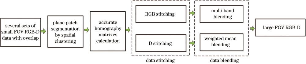
Fig. 1. Flow chart of RGB-D data stitching

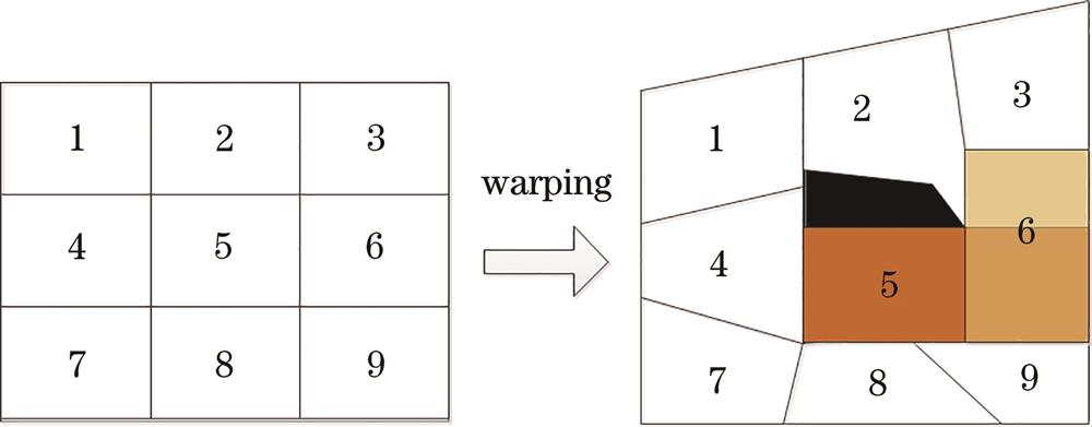
Fig. 2. Super-pixel warping

Fig. 3. Schematic of overlap interpolation

Fig. 4. Schematic of black hole interpolation

Fig. 5. Small FOV RGB-D data acquired under four viewpoints. (a) The first view RGB image; (b) the first view depth map; (c) the second view RGB image; (d) the second view depth map; (e) the third view RGB image; (f) the third view depth map; (g) the fourth view RGB image; (h) the fourth view depth map

Fig. 6. Large FOV RGB image

Fig. 7. Spatial information clustering results of RGB-D data in RGB images and depth images of the first view and the fourth view. (a) Result of the first view RGB image segmentation; (b) result of the first view depth image segmentation; (c) result of the fourth view RGB image segmentation; (d) result of the fourth view depth image segmentation

Fig. 8. Depth map segmentation results with different number of sub-blocks. (a) 20 blocks; (b) 100 blocks

Fig. 9. Depth map segmentation result with α=1

Fig. 10. Depth map segmentation results with different β. (a) β=0.1; (b) β=8.5; (c)(d) corresponding local enlargement

Fig. 11. Comparison of overlap and black hole interpolations. (a) Overlap and black hole after direct coordinate transformation; (b) result obtained by only overlap interpolation; (c) result obtained by overlap and black hole interpolations

Fig. 12. Results of RGB-D data stitching based on spatial information clustering. (a) Result of RGB image stitching; (b) result of depth image stitching

Fig. 13. Result of RGB stitching based on global homography transformation

Fig. 14. Results of image stitching with different number of grids. (a) 49 grids; (b) 1600 grids

Table 1. Quantitative evaluation of different methods