Fig. 1. Schematic setup for laser speckle contrast imaging (LSCI)^[30]

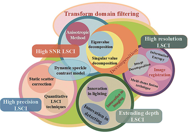
Fig. 2. Analysis and solution of key technical problems of LSCI

Fig. 3. Scheme of aLSCI algorithm^[98]

Fig. 4. Comparative experimental results of different algorithms^[98]. (a) tLSCI algorithm; (b) sLSCI algorithm; (c) stLSCI algorithm; (d) savgtLSCI algorithm; (e) tavgsLSCI algorithm; (f) aLSCI algorithm; (g) contrast-to-noise ratio (CNR) of different algorithms

Fig. 5. LSCI filtering model based on eigenvalue-decomposition^[64] (X': original speckle signal vector; X: speckle signal vector after denoising; XS: static scattered light signal; XB: fluctuating blood signal; XW: white noise signal)

Fig. 6. LSCI filtering algorithm based on eigenvalue-decomposition and filtering^[100]

Fig. 7. Comparative experimental results^[100]. (a) Raw fundus contrast image; (b) fundus contrast image after eigenvalue-decomposition and spatial filtering

Fig. 8. Scheme of MD-ABM3D algorithm^[47]

Fig. 9. Output of different denoising algorithms^[47]. (a) Original image, where PSNR is 18.5, MSSIM is 0.46, and R is 0.813; (b) savg-tLSCI algorithm, where PSNR is 32.8, MSSIM is 0.87, and R is 0.987; (c) NLM algorithm, PSNR is 31.0, MSSIM is 0.90, and R is 0.986; (d) BM3D algorithm, PSNR is 35.8, MSSIM is 0.92, and R is 0.993; (e) MD-ABM3D algorithm, PSNR is 37.8, MSSIM is 0.96, and R is 0.996; (f) reference image

Fig. 10. Model of rLASCA algorithm^[61]

Fig. 11. Experimental results of rLASCA algorithm^[61]. (a) Unregistered laser speckle contrast image; (b) laser speckle contrast image registered by rLASCA; (c) enlarged image of white rectangular box area in figure (a); (d) enlarged image of white rectangular box area in figure (b); (e) white light map of white rectangular box area

Fig. 12. Non-rigid registration algorithm based on non-coherent light^[45]. (a) Experimental setup of dual-mode lighting system; (b) algorithm model

Fig. 13. Comparison of rigid registration and non-rigid registration^[45]. (a) Unregistered blood flow image; (b) blood flow image after rigid registration; (c) blood flow image after non-rigid registration

Fig. 14. Correction model for LSCI movement artifact based on image decomposition^[106]. (a) Correction model; (b) selection of regression variance; (c) fitted by regression analysis; (d)-(f) contrast value before and after movement correction

Fig. 15. LSCI correction model based on contourlet transform and multi-focus image fusion^[46]

Fig. 16. Experiment results before and after nonuniform intensity correction^[103]. (a) Contrast image affected by nonuniformity; (b) reconstructed contrast image

Fig. 17. Experimental results of nonuniform correction^[110]. (a) Grayscale speckle images at two different intensities; (b) from the top to the bottom: contrast maps at high intensity and low intensity and corrected contrast map at low intensity; (c) contrast profile along the red line marked in figure (a) of contrast maps at low intensity and high intensity and corrected contrast map at low intensity; (d) contrast profile along yellow line marked in figure (a) of corrected contrast map at low intensity

Fig. 18. Blood flow image processed by dLSI algorithm^[84]

Fig. 19. Schematic of multi-focus imaging setup^[119]

Fig. 20. Model of dynamic scattering contrast correction model^[74]

Fig. 21. Spatial frequency domain imaging^{LSCI[121]. (a) Experimental setup of si-SFDI; (b) processing flow of si-SFDI}

Fig. 22. Experimental setup for optical speckle image velocimetry (OSIV)^[10]

Fig. 23. Processing flow of OSIV algorithm^[10]

Fig. 24. Sample entropy-based laser speckle contrast analysis method and partial experimental results^[111]. (a) Sample entropy-based laser speckle contrast analysis method; (b) partial experimental results

Fig. 25. Multi-exposure laser speckle imaging^[83]. (a) Multi-exposure speckle imaging system; (b) percentage deviation in τc under single exposure model and MESI

Fig. 26. Lateral speckle contrast analysis method combined with non-wide field illumination^[127]. (a) Schematic of LSCI experimental setup based on line beam scanning illumination; (b) image processing flow; (c)-(d) blood flow images obtained by traditional contrast analysis method, lateral speckle contrast analysis methods weighted with constant and depth sensitivity curves, respectively

Fig. 27. Schematic of DSCA imaging system^[132]

Fig. 28. LSCI system for blood flow^[130]. (a) TR-LSCI system; (b) conventional reflective-detected LSCI system

Fig. 29. Novel LSCI systems and their advances in application and research

Fig. 30. Portable LSCI based on DSP^[135]. (a) Schematic illustration of portable LSCI system; (b) block diagram of hardware framework; (c) block diagram of software framework

Fig. 31. Portable LSCI based on FPGA^[136]

Fig. 32. Efficient portable LSCI based on embedded GPU^[57]

Fig. 33. Endoscopic LSCI system^[50,88]

Fig. 34. Dual-display laparoscopic laser speckle contrast imaging (LSCI) system^[14]. (a) Laparoscopic LSCI system; (b) inserted laparoscopy; (c) handheld operation; (d) LSCI bowel imaging; (e) LSCI gallbladder imaging; (e) LSCI mesentery imaging

Fig. 35. Head-mounted LSCI^[60]

Fig. 36. Schematic of ECoG-LSCI^[23]

Fig. 37. Speckle contrast images for rCBF upon electrical stimulation in forelimb- and hindlimb-stimulated groups at serial time points^[23]

Fig. 38. Multimodal and functional imaging of retina^[17]

Fig. 39. Multimodal system for real-time surgical guidance^[141]

Table 1. Correction model of dynamic speckle contrast^[115]

Table 2. Electric field autocorrelation function g1τ for different scattering characteristics and particle motion models^[73]