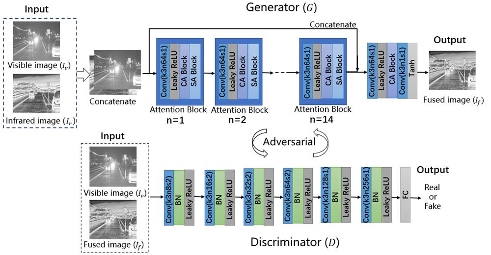
Fig. 1. Architecture of the proposed EAGAN. CA Block：channel attention block，SA Block：spatial attention block，BN：batch normalization，FC：fully connected layer，Conv：corresponding kernel size（k），number of feature maps（n）and stride（s）indicated for each convolutional layer

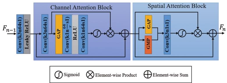
Fig. 2. Architecture of Attention Block. GAP：Global Average Pooling，GMP：Global Max Pooling，r：scaling factor，Conv：corresponding kernel size（k），number of feature maps（n）and stride（s）indicated for each convolutional layer

Fig. 3. Qualitative comparison of different algorithms on 4 typical infrared and visible image pairs. From top to bottom：visible image，infrared image，fusion results of ASR，GFF，GTF，DenseFuse，FusionGAN，RCGAN and our algorithm.

Fig. 4. Qualitative comparison of different algorithms on 5 typical infrared and visible image pairs from TNO dataset. From left to right：Duine sequence，Nato_camp_sequence，Kaptein_1123，men in front of house and soldier_behind_smoke_3. From top to bottom：visible image，infrared image，fusion results of ASR，GFF，GTF，DenseFuse，FusionGAN，RCGAN and our algorithm.

Fig. 5. Qualitative comparison of different algorithms on 4 typical infrared and visible image pairs from INO dataset. From left to right：ParkingSnow，GroupFight，MultipleDeposit，ClosePerson. From top to bottom：visible image，infrared image，fusion results of ASR，GFF，GTF，DenseFuse，FusionGAN，RCGAN and our algorithm.

Fig. 6. Attention weight maps：（a）the infrared image；（b）the visible image；（c）the fused result of our proposed EAGAN；（d）Output result of the third attention block；（e）Channel Attention weight map；（f）Spatial Attention weight map

Fig. 7. The effect of attention mechanism on fusion results：（a）fusion result of the network without attention mechanism；（b）fusion result of our algorithm.

Fig. 8. Fusion results when the loss function of the generator changes：（a）ℒG=λ1ℒperceptual；（b）ℒG=λ2ℒedge；（c）ℒG=ℒEAGANG；（d）ℒG=ℒEAGANG+λ1ℒperceptual；（e）ℒG=ℒEAGANG+λ2ℒedge；（f）ℒG=λ1ℒperceptual+λ2ℒedge；（g）result of EAGAN.

Table 1. Quantitative comparison of different algorithms on RoadScene dataset

Table 2. Quantitative comparison of different algorithms on TNO dataset

Table 3. Quantitative comparison of different algorithms on INO dataset

Table 4. Comparison of effects of attention mechanism on fusion results