
Sheng Huang, Feifei Li, Qiu Chen. Computed Tomography Image Classification Algorithm Based on Improved Deep Residual Network[J]. Acta Optica Sinica, 2020, 40(3): 0310002
- Acta Optica Sinica
- Vol. 40, Issue 3, 0310002 (2020)
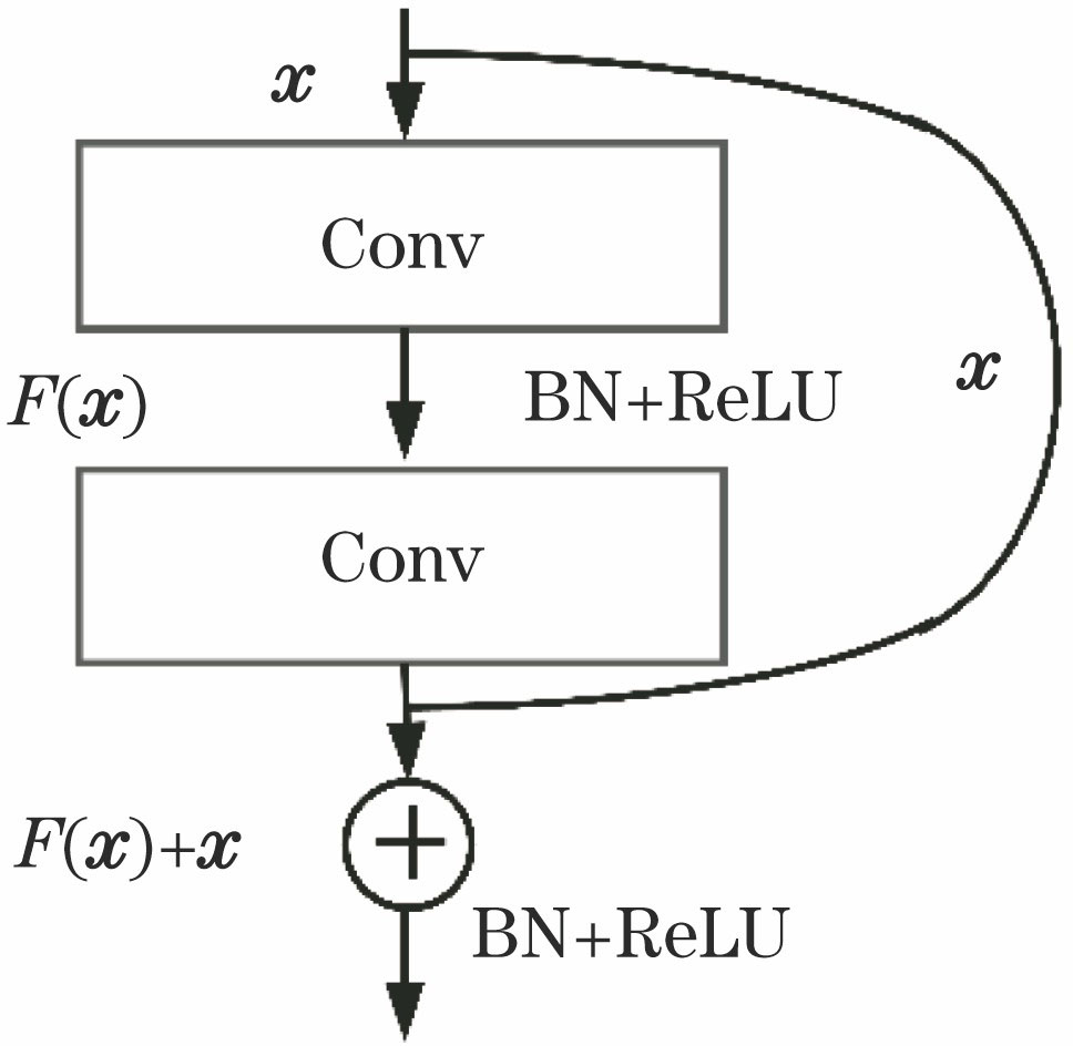
Fig. 1. Residual block
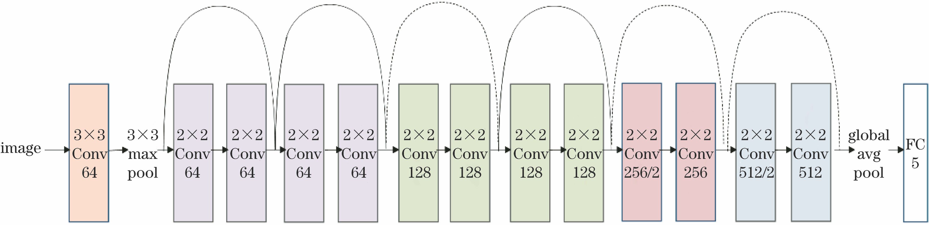
Fig. 2. Architecture of SK-ResNet
Fig. 3. Structure of discriminator
Fig. 4. Process of unsupervised pre-training
Fig. 5. Example of labeled areas of lung (areas 1, 2 denote pathology area)
Fig. 6. Image patch examples. (a) Source domain; (b) target domain
Fig. 7. Trend graph of classification results for training sets with different scales
Fig. 8. Misclassified examples
|
Table 1. Different dataset separation schemes
| ||||||||||||||||||||||||||||
Table 2. Comparison of classification results of SK-ResNet with different depths
|
Table 3. Comparison of results on SK-ResNet before and after using transfer learning
| |||||||||||||||||||||||||||||||||||||||||
Table 4. Classification confusion matrix of SK-ResNet
| |||||||||||||||||||||||||||||||||||||||||
Table 5. Classification confusion matrix of SK-ResNet using transfer learning
|
Table 6. Comparison of classification performances of SK-ResNet and other methods

Set citation alerts for the article
Please enter your email address
© Copyright 2018-2021 | Chinese Laser Press. All Rights Reserved 沪ICP备15018463号-20