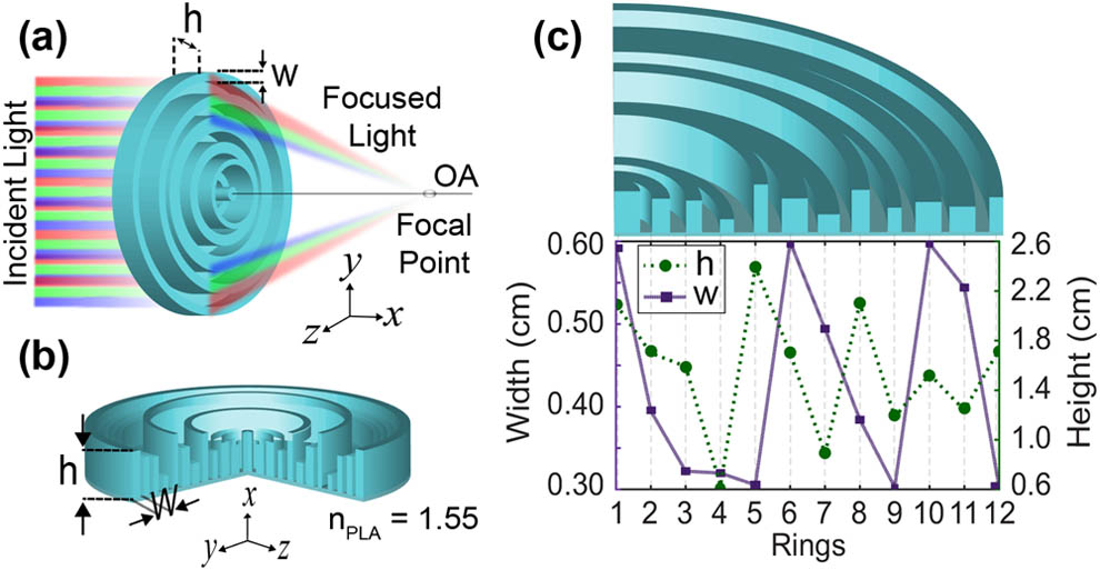
Fig. 1. (a) Schematic representation of planned AMDL with light-focusing behavior and optimization parameters. (b) Perspective view of designed AMDL consisting of PLA and (c) the quarter-cross sectional view of the lens with the plot of height and width for each ring.

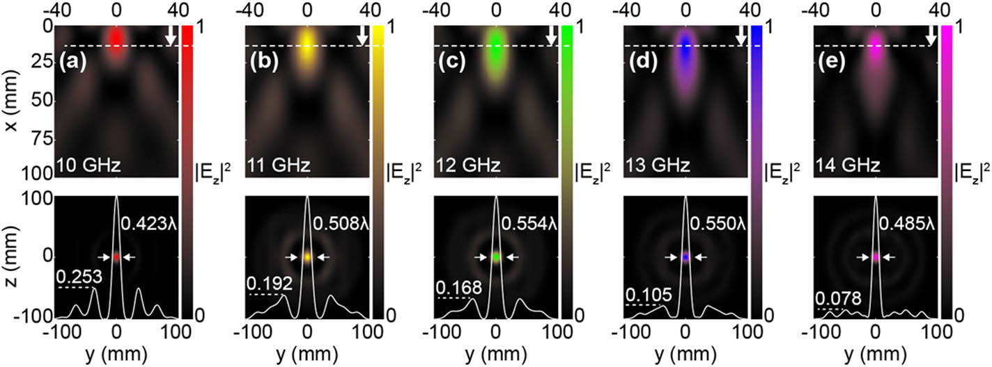
Fig. 2. Numerically calculated electric field intensity distributions (top) and calculated intensity distributions around the focal points with their lateral cross-sectional profiles and corresponding FWHM and MSLL values (bottom) at (a) 10 GHz, (b) 11 GHz, (c) 12 GHz, (d) 13 GHz, and (e) 14 GHz. The white horizontal dashed line indicates the desired focal distance (ΔFd=13.82  mm), and the white arrows indicate the propagation direction.

Fig. 3. Map of cross-sectional electric field intensity distributions in (a) longitudinal direction on the optical axis and (b) lateral direction at focal points. The black vertical dashed line represents a desired focal distance (ΔFd=13.82  mm). (c) The plot of back focal distance (ΔF) in mm (red solid) and FWHM (blue dashed). The blue solid line indicates the diffraction-limited FWHM values. (d) The focusing efficiency (red solid) and NA (blue dashed) graphs of selected frequency interval.

Fig. 4. Photograph of the 3D printed AMDL from (a) perspective and (b) top views. (c) Photographic view of the experimental setup. (d) Schematic representation of experimental setup to scan electric field intensity distributions at back focal plane (xz-plane: Scanning Area I) and around the focal point (zy-plane: Scanning Area II). Experimentally measured field intensity profiles (top) and measured intensity distributions around the focal points (bottom) at (e) 10 GHz, (f) 11 GHz, (g) 12 GHz, (h) 13 GHz, and (i) 14 GHz. The white horizontal dashed line indicates the desired focal distance (ΔFd=13.82  mm), and the white arrows indicate the propagation direction.

Fig. 5. Maps of experimentally measured cross-sectional intensity profiles (a) on the optical axis and (b) at focal points. The black vertical dashed line represents desired focal distance (ΔFd=13.82  mm). (c) Graphs of both ΔF and FWHM values. (d) Focal distances at the frequency region between 12 and 13 GHz [the zoom-out frequency region of the shaded area in plot (c)].

Fig. 6. (a) Quarter-cross sectional view of the nano-scaled lens with the plot of height and width for each zone. (b) Map of cross-sectional intensity profiles on optical axis, (c) plots of both ΔF and focusing efficiency, and (d) graphs of both NA and FWHM values with respect to operating wavelengths of 380 and 620 nm.

Fig. 7. Numerically calculated electric field intensity distributions with 40-nm-wavelength steps at (a) 380 nm, (b) 420 nm, (c) 460 nm, (d) 500 nm, (e) 540 nm, (f) 580 nm, and (g) 620 nm. The dashed lines represent the average focal distance (233 nm).

Table 1. Numerical and Experimental Characteristics of AMDL with Their Average Values