Ultra-compact, high-numerical-aperture achromatic multilevel diffractive lens via metaheuristic approach

Bumın K. Yildırım; Hamza Kurt; Mirbek Turduev

doi:10.1364/PRJ.427523

Abstract

Recently, multilevel diffractive lenses (MDLs) have attracted considerable attention, mainly due to their superior wave-focusing performance; however, efforts to reduce chromatic aberration are still ongoing. Here, we present a numerical design and experimentally demonstrate a high-numerical aperture (

\sim 0.99

), diffraction-limited achromatic multilevel diffractive lens (AMDL), operating in the microwave range of 10–14 GHz. A multi-objective differential evolution (MO-DE) algorithm was incorporated with the three-dimensional (3D) finite-difference time-domain method to optimize the heights and widths of each concentric ring (zone) of the AMDL structure. To the best of our knowledge for the first time, in this study, the desired focal distance was also treated as an optimization parameter in addition to the structural parameters of the zones. Thus, MO-DE diminishes the necessity of predetermined focal distance and center wavelength by also providing an alternative method for phase profile tailoring. The proposed AMDL can be considered an ultra-compact and flat lens since it has the radius of

3.7 λ_{c}

and a thickness of

\sim λ_{c}

, where

λ_{c}

is the center wavelength of 24.98 mm (i.e., 12 GHz). The numerically calculated full width at half maximum values are

< 0.554 λ

and focusing efficiency values are varying between 28% and 45.5%. To experimentally demonstrate the functionality of the optimized lens, the AMDL composed of polylactic acid material polymer is fabricated via 3D-printing technology. The numerical and experimental results are compared, discussed in detail, and observed to be in good agreement. Moreover, the verified AMDL in the microwave regime is scaled down to the visible wavelengths to observe achromatic and diffraction-limited focusing behavior between 380 and 620 nm wavelengths.

1. INTRODUCTION

One of the most fundamental manipulations of light is its focusing/gathering to a desired location in space [1]. However, optical aberrations, both monochromatic and chromatic, still represent a major hurdle in this endeavor [2]. Chromatic aberration is the phenomenon where the dependence of the material refractive index on wavelength causes the light of different wavelengths to focus on different points in space [3,4]. The creative endeavors to reduce chromatic dispersion started with achromatic doublets in the 18th century [5], followed by applying hybrid refractive–diffractive lenses [6,7] and graded-index optics [8].

In addition, contemporary studies have presented several solutions to overcome chromatic dispersion. The most common methods to design meta-lenses are tailoring the phase profiles [9 –13], combining meta-surfaces with refractive devices as a hybrid structure to balance the material dispersion [14], manipulating the polarization rotation of incident light [15], and meta-surfaces doublets [16]. Additionally, multilevel diffractive lenses (MDLs) provide not only achromatic focusing, but also polarization-insensitive, broadband, and energy efficient focusing with their reduced weight and size compared to the meta-lenses [17 –21]. In the MDL structures, each zone (concentric ring) plays an important role in reducing chromatic aberration provided that the zone’s parameters are adjusted properly [22]. Hence, various optimization and inverse design methods have been exploited to obtain appropriate MDL parameters for efficient focusing [23 –26]. One of the important design characteristics of meta-lenses and MDLs is their numerical aperture (NA) value, which is a function of focal length, the radius of the lens, and the refractive index of the medium. It is difficult to obtain both a high NA value and chromatic aberration-free focusing [27]; however, an appropriate MDL design can overcome low efficiency and chromatic dispersion problems of the meta-lenses [28,29].

In this paper, we present a high-NA, diffraction-limited broadband achromatic multilevel diffractive lens (AMDL) operating in the microwave regime between 10 and 14 GHz. A multi-objective differential evolution (MO-DE) algorithm is applied to minimize chromatic aberration and maximize the AMDL focusing efficiency by tightly confining the diffracted light energy in the main lobe and suppressing the side lobes (suppression of the side lobes is aimed at achieving a clear and efficient focal spot). Here, the heights and the widths of each AMDL zone are optimized to achieve a predefined objective function. Moreover, differently from the proposed achromatic meta-lens and MDL designs in the literature, in this study, the focal distance is directly optimized by the algorithm without fixing it to the desired center frequency (fixing of the center frequency is an important requirement for phase profile engineering in achromatic lens designs). In other words, this approach diminishes the necessity of determining focal distance and center wavelength and provides an alternative way to engineer phase profiles. In addition, to experimentally verify the numerical results, measurements in the microwave regime were performed by fabricating proposed AMDL using 3D-fused deposition modelling (3D-FDM) with polylactic acid (PLA) material. We also scaled down the optimized AMDL to the visible wavelengths by taking 550 nm as a reference wavelength ( $λ_{ref}$ ) to observe the achromatic focusing behavior. All AMDL characteristics of wavelengths in the range 380–620 nm were investigated in detail in the discussion section.

Sign up for Photonics Research TOC. Get the latest issue of Photonics Research delivered right to you！Sign up now

2. DESIGN METHODOLOGY AND NUMERICAL RESULTS OF AMDL

In this study, the differential evolution (DE) algorithm is used to obtain an ultra-compact, high-NA and broadband functional achromatic MDL. DE is a metaheuristic approach that provides sufficiently appropriate solutions to multi-objective optimization problems by taking advantage of the biological mechanisms such as cross-over, mutation, and selection of natural evolution process [30]. It is important to note that in our previous works, we have successfully applied the DE algorithm in various photonic and optic applications [4,31 –33]. The DE algorithm iteratively converges to a desired target, which is defined as a cost function. The searching ability of DE depends on the defined heuristic mechanism and objective function. Initially, the optimization algorithm starts with a fixed number ( $μ$ ) of randomly generated individuals, namely MDL structures (structures under analysis) having randomly modulated the heights and widths of each zone. The number of individuals of a generation (iteration) is constant. In our study, the number of vector population ( $μ$ ) is 20. It means that in every iteration (including initialization), 20 randomly created lens structures are simulated for randomly determined focal distances, and the cost values are calculated. The term “randomly” refers to the random assignment of each parameter for every 20 individuals.

Before the population can be initialized, both upper ( $b^{U}$ ) and lower ( $b^{L}$ ) limits of each parameter ( $x_{i}$ ) are determined by using Eq. (1) [30]: $x_{i} = {rand}_{i} (0, 1) \times (b_{i}^{U} - b_{i}^{L}) + b_{i}^{L} .$ (1)Here, $x$ represents an individual in the population ( $μ$ ), and subscript $i$ indicates the randomly generated parameter ( $i = 1, \dots, D$ ). The number of parameters ( $D$ ) is 25. The first 12 parameters are used for the widths of each zone, parameters 13–24 are used for the heights of each zone, and the last parameter is assigned to the desired focal length value.

Following the algorithm initialization, i.e., after initial population is generated, we select three different individuals from the instant generation where one of them is the best individual of the corresponding generation. These three vectors are used to create one mutated individual, which is defined as mutation mechanisms. The mutation mechanisms are implemented to generate $μ$ mutated individuals. So far, we have $μ$ instant individuals (parents) and $μ$ mutated individuals. Later, the crossover mechanism takes part to generate a new individual (children). We apply the crossover mechanism repeatedly to generate $μ$ new individuals. The selection of best individual for the basis vector is essential. Here, the selection mechanism plays an important role in transferring individuals to next generation. Formerly, we generated new individuals, and the number of individuals was increased to $2 μ$ . Here, we should apply a selection algorithm to eliminate $μ$ individuals to reduce the number of individuals to $μ$ again, which is a necessary condition for the operation of an evolutionary algorithm. One can easily select the new individuals (children) to survive and eliminate the parents. The idea behind this selection mechanism, which also applies the elitism criterion, is that the relatively good individuals are transferred to next generation. One of the eliminated parents could be better than one of the children who survived, which provides algorithm to rationally spread over the search space. We have terminated the algorithm when it did not provide a better solution for several iterations. In addition, one can restrict the operation of an algorithm to a predefined number of iterations. Furthermore, one can terminate the algorithm as the speed of convergence reduces to a predefined limit.

The MO-DE optimization algorithm is embedded into a three-dimensional (3D) finite-difference time domain (FDTD) [34] method to design an ultra-compact, high-NA and achromatic MDL. Figure 1(a) illustrates the AMDL structure intended for design with its structural parameters [i.e., heights ( $h$ ) and widths ( $w$ )] and achromatic focusing strategy, where the colored parallel lines refer to polychromatic light excitation. Here, MO-DE optimizes these parameters (i.e., $h$ and $w$ are determined by the DE algorithm) to reveal both achromatic (focusing of polychromatic light into a particular point) and diffraction limited focusing [forcing both the full width at half maximum (FWHM) and maximum side-lobe level (MSLL) values to decrease] by using user-defined multi-objective cost function, whose analytical expression is given in Eq. (2): $f_{cost} = w_{1} \times \sum_{i = 1}^{n} FWHM (λ_{i}) + w_{2} \times \sum_{i = 1}^{n} MSLL (λ_{i}) + w_{3} \times \sum_{i = 1}^{n} | Δ F (λ_{i}) - Δ F_{d} | + w_{4} \times \sum_{i = 1}^{(n - 1) / 2} | Δ F (λ_{n - i + 1}) - Δ F (λ_{i}) | .$ (2)Here $w_{1}$ , $w_{2}$ , $w_{3}$ , and $w_{4}$ values are the weights assigned to each goal in the function. The exact values of the weighting factors should be assigned before the optimization process. To determine the appropriate objective function with consistent weighting factors, trial simulations were performed. The first and second terms of the function are related to the AMDL focusing performance, and the remaining terms are responsible for correcting the focusing chromaticity issue by equalizing all back focal distances of the different wavelengths. In Eq. (2), $FWHM (λ_{i})$ and $MSLL (λ_{i})$ are the FWHM and MSLL values of each wavelength $(λ_{i})$ corresponding to microwave frequency regime 10–14 GHz. Within this frequency interval 15 equally distant frequency (i.e., $n = 15$ different wavelengths) points are chosen for $f_{cost}$ calculation. $Δ F (λ_{i})$ represents the back focal distance of the $i$ th wavelength, and $Δ F_{d}$ is the desired focal length. Here, desired focal distance $Δ F_{d}$ is determined by the MO-DE algorithm during the optimization process. It is important to note that the extremum values of $Δ F_{d}$ , which can be taken by the MO-DE algorithm, lie between $0.2 λ_{c}$ and $1 λ_{c}$ (this interval is defined by considering near-field focusing and to achieve high NA), where $λ_{c}$ is the center wavelength (i.e., 12 GHz frequency). This is a very important difference from other achromatic lens design strategies described in the literature [12 –20,25 –29] because here the optimization method decides where the better focal point location is beneficial for achieving an achromatic focusing effect. In short, the aim of the optimization algorithm is to minimize the $f_{cost}$ function by reducing FWHM and MSLL values for all frequency ranges and focusing all wavelengths into the same focal point, which is decided by MO-DE.

(a) Schematic representation of planned AMDL with light-focusing behavior and optimization parameters. (b) Perspective view of designed AMDL consisting of PLA and (c) the quarter-cross sectional view of the lens with the plot of height and width for each ring.

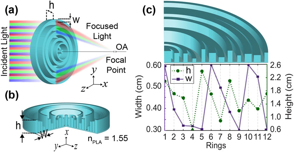
Figure 1.(a) Schematic representation of planned AMDL with light-focusing behavior and optimization parameters. (b) Perspective view of designed AMDL consisting of PLA and (c) the quarter-cross sectional view of the lens with the plot of height and width for each ring.

We also note that one can use our approach to design an achromatic lens with the fixed focal length. However, optimizing the focal length value plays a crucial role in the mitigation of chromatic aberration, especially when intended lens design has limits on the geometrical parameters due to available fabrication and characterization facilities, like in the case of proposed AMDL. Optimizing focal distance becomes more important if the design approach is based on heuristics rather than exact analytical design, like in the case of conventional diffractive lenses. In our opinion, proposed design approach, where focal distance is not fixed but optimized, is beneficial for improving the achromatic performance of the MDL structures.

The designed lens is composed of PLA material, which has a low permittivity value $ε_{PLA} = 2.4025$ in the microwave region. This PLA material is preferred for the following reasons: PLA is a thermoplastic material, which is with very low loss, or effectively lossless, dielectric material in the microwave region [35,36]. It means that the possible attenuation caused by the material absorption can be neglected. In addition, the PLA material was cost efficient to fabricate the designed AMDL and perform microwave experiments. The number of zones whose structural dimensions vary is fixed to 12. This number is intentionally chosen considering fabrication limitation of the 3D printing physical area, limited to $29 cm \times 19 cm \times 16 cm$ (physical area of the printing of “MakerBot Replicator +” 3D printer). Moreover, the ranges of values of the zones’ heights and widths that can be defined by the MO-DE are changing from 3 to 6 mm and from 6 to 26 mm, respectively. Finally, after the exact definition of the multi-objective function, the MO-DE is integrated with 3D FDTD, and optimization is performed. The final optimized AMDL is presented in Fig. 1(b) and the optimization process is nearly 200 iterations (completed in approximately 14 days). Moreover, during the optimization of the structural parameters, the numerical modeling and time-domain analysis of the AMDL in each iteration were carried out by the 3D FDTD method. The computational simulations are done by running the computer system having the following hardware specifications: 3.6 GHz, Intel i9-9900K, 16 MB Smart Cache CPU, 8 cores, 64 GB RAM, 512 GB SSD. Furthermore, the memory requirement of the simulations in each iteration does not exceed 8 GB in this study, and the CPU having multi-core processors is enough for running FDTD simulations with an acceptable resolution of the computational domain. In all numerical simulations, the computational domain is a bounded 3D spatial domain, and undesired back reflections are absorbed by perfectly matched layers located at the boundaries of the computational domain [37]. During the optimization process to calculate $f_{cost}$ , the generated structures in each iteration are excited with a broadband transverse-magnetic (TM) polarized continuous sources with a Gaussian profile. We should note that the notation for TM polarization is defined as follows: the magnetic field is in the $x y$ -plane ( $H_{x}$ , $H_{y}$ ), and the electric field $E_{z}$ is perpendicular to the $x y$ -plane.

The MO-DE minimizes $f_{cost}$ function to achieve a high NA and achromatic MDL structure by optimizing the heights and widths of each zone. The parameters of each zone are presented in Figs. 1(b) and 1(c), respectively. The ultimate radius and thickness values of the AMDL emerged as 9.3 and 2.6 cm, where the substrate thickness is fixed to 0.2 cm. The substrate is required to hold optimized zones to generate AMDL. As can be seen from Fig. 1(c), the final values of zone widths vary between 0.30 and 0.59 cm, while the corresponding heights change from 0.63 to 2.40 cm. The MO-DE algorithm determined the desired focal length $(Δ F_{d})$ as 13.82 mm ( $0.553 λ_{c}$ , where $λ_{c} = 24.98 mm$ corresponds to 12 GHz frequency). As a result, the optimization attempted to focus all wavelengths into the desired focal distance of 13.82 mm. Moreover, it also tried to increase the focusing performance of AMDL for all wavelengths (between 10 and 14 GHz) by preserving achromatic focusing effect.

Figure 2 shows the numerically calculated steady-state spatial electric field intensity ( ${| E_{z} |}^{2}$ ) profiles of the focused beam in the $x y$ - and $z y$ -planes for different operating frequencies. In Figs. 2(a)–2(e) the electric field intensity distributions (depicted in top line) in the $x y$ -plane at the frequencies of 10–14 GHz with a 1 GHz step are presented, respectively. Here, numerically calculated back focal distances are 9.92 mm and 13.27 mm for 10 GHz and 11 GHz, respectively. In contrast, the AMDL focuses light at operating frequencies of 12, 13, and 14 GHz to the same back focal distance of 14.42 mm. Similarly, in Figs. 2(a)–2(e) the plots given in the bottom row illustrate the focal spot (field concentration) of calculated electric field intensity at the selected frequency points in the $z y$ -plane. The normalized lateral cross-sectional profiles of focal spot in the $z y$ -plane are also superimposed in these plots. As can be seen from Figs. 2(a)–2(e), the calculated FWHM values of focused beam vary between $0.423 λ$ and $0.554 λ$ , where $λ$ denotes the wavelength of each selected frequency, while the corresponding MSLL values change between 0.078 and 0.253, which means that most of the energy is confined in the focal spot (i.e., main lobe). If we look at the results presented in Fig. 2, we can see that the MO-DE succeeded to focus the light near self-defined $Δ F_{d}$ focusing distance of 13.82 mm. For instance, for operating frequencies of 10 GHz and 11 GHz the differences between self-defined (optimized) $Δ F_{d}$ and obtained focal distances are $0.156 λ_{c}$ and $0.022 λ_{c}$ , respectively. Furthermore, for the remaining frequencies (12, 13, and 14 GHz), the shift from the $Δ F_{d}$ is $0.022 λ_{c}$ , where $λ_{c} = 24.98 mm$ . From the given results, we can see that the implemented optimization method accomplished a strong focusing of light (FWHMs are near $0.5 λ$ ) and achromatic focusing with the average shift in focal lengths of 2.2% for the frequencies of 11, 12, 13, and 14 GHz [25].

Figure 2.Numerically calculated electric field intensity distributions (top) and calculated intensity distributions around the focal points with their lateral cross-sectional profiles and corresponding FWHM and MSLL values (bottom) at (a) 10 GHz, (b) 11 GHz, (c) 12 GHz, (d) 13 GHz, and (e) 14 GHz. The white horizontal dashed line indicates the desired focal distance ( $Δ F_{d} = 13.82 mm$ ), and the white arrows indicate the propagation direction.

To analyze the broadband operation and performance of the designed AMDL, Fig. 3 was prepared. The maps of cross-sectional electric field intensity ( ${| E_{z} |}^{2}$ ) profiles in longitudinal direction and the lateral direction at the focal point location are given in Figs. 3(a) and 3(b), respectively. The dashed line superimposed to the map in Fig. 3(a) defines the location of $Δ F_{d}$ . Moreover, both maps in Figs. 3(a) and 3(b) demonstrate the strong focusing effect with corrected chromaticity through the broadband frequency regime, except at the frequencies around 12.5 GHz, where the focused light is slightly shifted from the dashed line.

$Map of cross-sectional electric field intensity distributions in (a) longitudinal direction on the optical axis and (b) lateral direction at focal points. The black vertical dashed line represents a desired focal distance (ΔFd=13.82 mm). (c) The plot of back focal distance (ΔF) in mm (red solid) and FWHM (blue dashed). The blue solid line indicates the diffraction-limited FWHM values. (d) The focusing efficiency (red solid) and NA (blue dashed) graphs of selected frequency interval.$

Figure 3.Map of cross-sectional electric field intensity distributions in (a) longitudinal direction on the optical axis and (b) lateral direction at focal points. The black vertical dashed line represents a desired focal distance ( $Δ F_{d} = 13.82 mm$ ). (c) The plot of back focal distance $(Δ F)$ in mm (red solid) and FWHM (blue dashed). The blue solid line indicates the diffraction-limited FWHM values. (d) The focusing efficiency (red solid) and NA (blue dashed) graphs of selected frequency interval.

There is a smooth transition from the general trend (being achromatic) to a wavelength-dependent focusing at around 12.5 GHz. Both the focal point and FWHM reach minimum values at this frequency, and the achromatic response is apparent as we continue tracing the rest of the bandwidth. It is surprising that the deployed algorithm generates an AMDL holding four zones and binary gratings of different heights and widths in a rather regular fashion. However, some of the structural parameters break the design rules of diffractive lens that can be used based on the analytical expressions [22]. Hence, even though it is difficult to identify the exact physical mechanism behind the characteristic observed at around 12.5 GHz, this behavior could be attributed to weakly guided resonance mode effect. When we calculated the transmission coefficient (plot skipped for simplicity), we observed a slight dip in the transmitted light (at exactly 12.68 GHz). It could be an indication of the light coupling to weakly guided mode in AMDL. By inspecting the field plots in the $x y$ -plane, $(w / c) \times n_{eff} \times D$ becomes integer multiples of $2 π$ at the resonance condition. The AMDL diameter is represented by $D$ . Finally, the spatial periodicity $Λ$ satisfies the condition $Λ ≪ λ$ so that the multi-level grating can be assumed as a subwavelength grating.

In Fig. 3(c), calculated focal distances ( $Δ F$ ) and FWHM values are plotted for the frequencies in the range 10–14 GHz. The minimum and maximum focal distance values are calculated as 9.92 mm and 15.02 mm, respectively, and the variation is only 5.10 mm, which almost equals $λ_{c} / 5$ . Here, $λ_{c}$ is the wavelength of the center frequency (12 GHz), which is 24.98 mm. The average value of the broadband $Δ F$ is 13.49 mm, which means that the average shift in focal lengths equals 2.38% [25]. All the presented results verify that the implemented MO-DE algorithm satisfactorily suppresses the focal shift over a broadband range. Furthermore, the calculated FWHM values are varying between $0.423 λ$ and $0.610 λ$ for the frequency interval between 10 and 14 GHz. We know that the theoretical diffraction limited FWHM of the focused light is $\sim λ / 2 \times NA$ , and we can see that in both smaller and larger frequency values, the designed AMDL surpasses this limit. To further analyze the focusing performance of AMDL within the frequency region of 10–14 GHz, NA and focusing efficiency values are calculated. Here, the focusing efficiency is calculated as the fraction of collected incident light on the focal plane with a radius equal to three times the FWHM spot size [38,39].

It is also important to quantitively analyze the broadband focusing performance of the proposed AMDL. For this purpose, the focusing efficiency and NA values were extracted and demonstrated in Fig. 3(d). Within the defined frequency interval, NA values are calculated as $> 0.986$ , and the focusing efficiency increases from 28% to 45.5%. As visible from the corresponding figure, the overall broadband focusing efficiency starts decreasing linearly after frequency of 12 GHz from 40% to 28%. From the light focusing map presented in Fig. 3(a), one can see that the light is tightly confined around the focal spots until 12 GHz; however, above 12 GHz, the overall energy is dispersed around the focal spot. Moreover, low focusing efficiency of the AMDL can be associated with a shadowing effect around the focal point, which mainly occurs due to the finite depth surface [40,41]. In other words, for the case AMDL structure, the discontinuities of the wrapped phase due to different heights of the zones, as well as the height difference between zones and substrate, lead to creation of a shadow that wastes light into undesired artificial orders [42,43].

It is important to note that the Strehl ratio is more relevant performance criteria than presenting the resolution in terms of FWHM [44]. For this reason, we calculated the Strehl ratio for the proposed AMDL, and an average Strehl ratio value emerged as 0.7174 for an operating frequency region between 10 and 14 GHz.

3. EXPERIMENTAL ANALYSIS OF ACHROMATIC FOCUSING EFFECT

To verify the operation principle and focusing performance of the designed AMDL, experiments were conducted in the microwave frequency region. The designed lens was produced using 3D–FDM with PLA thermoplastic polyester material. PLA is an all-dielectric, affordable, and biodegradable material that has a low dielectric constant value of $ε_{PLA} = 2.4025$ in the microwave range between 10 and 14 GHz. The designed AMDL is 3D printed using a commercially available “MakerBot Replicator +” 3D printer. Furthermore, the FDM of the 3D printer was set to fabricate the AMDL with a 100% infill ratio to generate the solid and homogeneous distribution of PLA material throughout the AMDL.

The photographic illustrations of the perspective and top views of the fabricated AMDL are presented in Figs. 4(a) and 4(b), respectively. Furthermore, the stand for the AMDL to allocate it straight [in parallel to the horn antenna that illuminates AMDL with microwave source, see Fig. 4(a)] is produced and is covered by microwave-absorbing materials to reduce the undesirable reflections. In the microwave experiments, an Agilent E5071C ENA vector network analyzer (VNA) was used to produce Gaussian profiled electromagnetic wave source through a horn antenna connected to VNA, whereas a monopole antenna was employed to scan the electric field distributions. The photographic illustration of the experimental setup and schematic view of the experimental measurements are presented in Figs. 4(c) and 4(d), respectively. In Fig. 4(d), a schematic of electric field distribution scanning areas is presented and defined as Scanning Area I for the $x z$ -plane and Scanning Area II for the $z y$ -plane. The electric field distributions of the corresponding scanning areas were measured using a motorized stage, which moves in $x z$ - and $z y$ -directions with the steps of 2 mm.

Figure 4.Photograph of the 3D printed AMDL from (a) perspective and (b) top views. (c) Photographic view of the experimental setup. (d) Schematic representation of experimental setup to scan electric field intensity distributions at back focal plane ( $x$ $z$ -plane: Scanning Area I) and around the focal point ( $z y$ -plane: Scanning Area II). Experimentally measured field intensity profiles (top) and measured intensity distributions around the focal points (bottom) at (e) 10 GHz, (f) 11 GHz, (g) 12 GHz, (h) 13 GHz, and (i) 14 GHz. The white horizontal dashed line indicates the desired focal distance ( $Δ F_{d} = 13.82 mm$ ), and the white arrows indicate the propagation direction.

Experimentally measured electric field distributions at the focal plane ( $x z$ -plane) with corresponding focal spot distributions ( $z y$ -plane) are presented in Figs. 4(e)–4(i) for the selected frequencies of 10, 11, 12, 13, and 14 GHz. In Fig. 4, the white dashed line defines optimized desired focal distance $Δ F_{d}$ position. Corresponding focal distances for the frequencies of 10, 11, 12, 13, and 14 GHz are 7.52, 10.57, 11.47, 19.65, and 16.96 mm, respectively. In addition, measured FWHM values remain $< 0.8 λ$ between 10 and 14 GHz. The normalized MSLL values are changing between 0.145 and 0.3827. The measured NA is $> 0.975$ for the frequency interval of 10–14 GHz. As seen in Fig. 4, the numerically calculated and experimentally measured focal distance values are not the same but show a similar tendency. Dissimilarity could be caused by the nonideal conditions of the experimental measurements: horn antenna might not generate exactly the same Gaussian profiled electromagnetic waves used in the FDTD simulations, for the impurity of the material, the production capability of the 3D printer, external factors such as temperature and imperfect alignment of the horn antennas. The experimentally measured results verify the overall functionality and efficient performance of the AMDL in terms of high NA and strong focusing effect, despite the small discrepancies in the focal distances.

To verify broadband operation functionality of the designed AMDL, the maps of the experimentally measured cross-sectional intensity profiles on the optical axis and on the lateral direction of focal point are presented in Figs. 5(a) and 5(b), respectively. The similarity in the numerical calculations and experimental measurements is evident, except for small shifts in the $Δ F$ values and a small decrease in the FWHM values. The quantitative demonstration of $Δ F$ and FWHM values can be seen in Fig. 5(c). The minimum and the maximum focal distance values are calculated as 7.50 mm and 20.9 mm, respectively, and the variation is only 13.40 mm, which almost equals $λ_{c} / 2$ , where $λ_{c}$ is the wavelength of the center frequency (12 GHz) and is 24.98 mm. The measured average value of the broadband $Δ F$ equals 12.85 mm, which means that the average shift in focal distances equals 7.01% [25]. As can be seen from Fig. 5(c), measured FWHM values are varying from $0.55 λ$ to $0.77 λ$ , which still shows a strong focusing effect of the proposed AMDL.

Figure 5.Maps of experimentally measured cross-sectional intensity profiles (a) on the optical axis and (b) at focal points. The black vertical dashed line represents desired focal distance ( $Δ F_{d} = 13.82 mm$ ). (c) Graphs of both $Δ F$ and FWHM values. (d) Focal distances at the frequency region between 12 and 13 GHz [the zoom-out frequency region of the shaded area in plot (c)].

It is important to note that the similar effect of a weakly guided resonance mode was not observed in the experimental results, as can be noticed in Fig. 5(a) (it is also evident in the zoom-out region that is given as an inset). For this reason, we prepared Fig. 5(d) to inspect in detail the focal shifts between 12 and 13 GHz. If we look at the extracted back focal distance values between 12 and 13 GHz presented in Fig. 5(d), we can see the abrupt deviation from the average focal distance starting from 12.4 GHz (shaded regions in the plot are given to emphasize the envelope of focal shift variations). In addition, there is a sharp deep in focal distance values between 12.5 and 12.7 GHz. This deviation and sharp deep in focal distances could be a sign of a weak resonance effect. However, we should note that these observations do not guarantee that we have the same resonance effect as in numerical results. In our opinion, a resonance effect may not be observed because of the possible slight difference in refractive indices of the AMDL material for simulations and experiments. Moreover, it is also impossible to meet the ideal computational domain conditions in experimental measurements like in simulations (presence of possible back-reflections and parasitic scatterings from the experimental environment).

It is difficult to directly measure the focusing efficiency of the AMDL through our microwave experimental setup; hence, we used an indirect method that resembles the numerical calculation [38,39] of the focusing efficiency of fabricated lens to provide comparable data. Here, the transmission value falling into a circular aperture with a radius equaling three times the FWHM centered at focal point is a proportioned transmission value falling into whole focal plane ( $200 mm \times 200 mm$ ). The obtained results are provided in Table 1. The experimentally measured focusing efficiency (F.E.) values are almost 10% below the numerically obtained values. The reason could be a larger size of the proportioned focal plane area than the lens coverage ( $186 mm \times 186 mm$ ), unlike 3D FDTD simulations.Table 1.

Numerical and Experimental Characteristics of AMDL with Their Average Values

Frequency (GHz)	3D FDTD					Experiment
Frequency (GHz)	$Δ F$ (mm)	FWHM ( $λ$ )	MSLL (n.i.)^a	NA	F.E. (%)	$Δ F$ (mm)	FWHM ( $λ$ )	MSLL (n.i.)^a	NA	F.E. (%)
10	9.92	0.423	0.253	0.994	45.55	7.52	0.562	0.351	0.997	32.19
11	13.27	0.508	0.192	0.990	38.23	10.57	0.635	0.382	0.994	30.14
12	14.42	0.554	0.168	0.988	39.94	11.47	0.590	0.275	0.992	26.03
13	14.42	0.550	0.105	0.988	35.41	19.65	0.726	0.230	0.979	23.18
14	14.42	0.485	0.078	0.988	27.91	16.96	0.575	0.277	0.983	22.35
Average	13.29	0.504	0.159	0.990	37.41	13.23	0.618	0.303	0.989	26.78

n.i., normalized intensity.

To compare the results of numerical calculation and experimental measurements, all data are collected in Table 1, and we can conclude that the experimental and numerical results are in good agreement with each other. Considering the average data (last column in Table 1), the NA values are almost the same in both cases. The differences in other parameters are within the acceptable ranges and might be caused by problems such as exciting the structure with a partial plane wave due to finite aperture size of the horn antenna and the misalignment of the antenna with the AMDL.

4. DISCUSSION

It is instructive to inspect the focusing performance of our optimized AMDL in the visible region. Unfortunately, due to the absence of an experimental facility, we could not carry out our analysis experimentally. Instead, we scaled the structural parameters of our designed AMDL to visible wavelengths to analyze its performance in the visible regime.

For this purpose, we chose 550 nm as a reference wavelength ( $λ_{ref} = 550 nm$ ) to scale down the AMDL, and the refractive index of the lens material was fixed to 1.467 for visible wavelengths [45]. The heights and widths of each AMDL zone are plotted in Fig. 6(a) with a quarter cross-sectional view. In this case, the overall radius of the lens and the thickness of the lens become 1.652 μm ( $3 λ_{ref}$ ) and 0.46 μm $(< λ_{ref})$ , respectively. The initial assigned distance between the closed edges of each zone emerges as 141 nm, as shown as an inset in Fig. 6(a). The achromatic focusing performance of the AMDL can be seen from the cross-sectional intensity map in Fig. 6(b). Although, the maximum deviation of focal points is calculated as 180 nm ( $\sim λ_{ref} / 3$ ), the back focal distances remain almost constant ( $\sim 270 nm$ ) at the wavelengths of 380–580 nm. In the range of wavelengths between 380 and 620 nm, the focusing efficiency values are linearly increasing from 28% to 60.7%. The calculated focal distance $(Δ F)$ and focusing efficiency values are superimposed in Fig. 6(c), whereas the NA values and FWHM values in the same wavelength interval are shown in Fig. 6(d). As expected, NA values are calculated above 0.985, and the FWHM values are almost equal to the corresponding diffraction-limited values. The FWHM values vary between $0.464 λ$ and $0.564 λ$ .

Figure 6.(a) Quarter-cross sectional view of the nano-scaled lens with the plot of height and width for each zone. (b) Map of cross-sectional intensity profiles on optical axis, (c) plots of both ΔF and focusing efficiency, and (d) graphs of both NA and FWHM values with respect to operating wavelengths of 380 and 620 nm.

The electric field intensity ( ${| E_{z} |}^{2}$ ) profiles of the focused beam in the $x y$ -plane for selected operating wavelengths starting from 380 nm and ending at 620 nm (with 40-nm-wavelength steps) are given in Figs. 7(a)–7(g). These fields also verify the achromatic focusing effect of the proposed AMDL. Here, numerically calculated back focal distances were deviating from 100 to 280 nm for the investigated visible wavelengths. The results show that the implemented optimization method accomplished the efficient focusing of light, as well as achromatic focusing with the average focal length of 233 nm for the wavelengths between 380 and 620 nm.

Figure 7.Numerically calculated electric field intensity distributions with 40-nm-wavelength steps at (a) 380 nm, (b) 420 nm, (c) 460 nm, (d) 500 nm, (e) 540 nm, (f) 580 nm, and (g) 620 nm. The dashed lines represent the average focal distance (233 nm).

5. CONCLUSION

This study demonstrated an all-dielectric achromatic MDL design operating between 10 and 14 GHz. The structural parameters of each AMDL zone were optimized through the 3D FDTD method, combined with a multi-objective differential evolution (MO-DE) algorithm. The optimized AMDL was fabricated via 3D-printing by using a low refractive index PLA ( $ε_{PLA} = 2.4025$ ) material to conduct microwave experiments for verification of the numerically obtained results. The fractional change between the average focal distances and the optimized desired focal length was measured numerically and experimentally as 2.2% and 7.01%, respectively. Furthermore, the focusing efficiency values were changing from 28% to 45% in numerical results. To numerically demonstrate the AMDL performance, simulations were performed between the wavelengths of 380 and 620 nm by scaling down the optimized AMDL. The designed AMDL also shows near-unity NA values over a broadband range. We believe that a proper design of this AMDL for visible and near infrared applications may provide excellent solutions for focusing issues in terms of efficient and aberration-free focusing.

Acknowledgment

Acknowledgment. H. Kurt acknowledges partial support from the Turkish Academy of Sciences. Authors would like to thank Jacob Engelberg from The Hebrew University of Jerusalem for his valuable comments and suggestions. H. Kurt acknowledges the financial support of KAIST Startup Funding (Project number G04200054).

References

[1] R. G. Gonzáles-Acuña, H. A. Chaparro-Romo, J. C. Gutiérrez-Vega. Analytical Lens Design(2020).

[2] E. L. Dereniak, T. D. Dereniak. Aberrations in optical systems. Geometrical and Trigonometric Optics, 292-322(2008).

[3] M. Born, E. Wolf. Principles of Optics(1980).

[4] B. K. Yildirim, E. Bor, H. Kurt, M. Turduev. Zones optimized multilevel diffractive lens for polarization-insensitive light focusing. J. Phys. D, 53, 495109(2020).

[5] R. Willach. New light on the invention of the achromatic telescope objective. Notes Rec. R. Soc. Lond., 50, 195-210(1996).

[6] W. Harm, C. Roider, A. Jesacher, S. Bernet, M. Ritsch-Marte. Dispersion tuning with a varifocal diffractive-refractive hybrid lens. Opt. Express, 22, 5260-5269(2014).

[7] S. Gorelick, A. de Marco. Hybrid refractive-diffractive microlenses in glass by focused Xe ion beam. J. Vac. Sci. Technol. B, 37, 051601(2019).

[8] R. Buczynski, A. Filipkowski, B. Piechal, H. T. Nguyen, D. Pysz, R. Stepien, A. Waddie, M. R. Taghizadeh, M. Klimczak, R. Kasztelanic. Achromatic nanostructured gradient index microlenses. Opt. Express, 27, 9588-9600(2019).

[9] F. Aieta, M. A. Kats, P. Genevet, F. Capasso. Multiwavelength achromatic metasurfaces by dispersive phase compensation. Science, 347, 1342-1345(2015).

[10] M. Khorasaninejad, Z. Shi, A. Y. Zhu, W. T. Chen, V. Sanjeev, A. Zaidi, F. Capasso. Achromatic metalens over 60 nm bandwidth in the visible and metalens with reverse chromatic dispersion. Nano Lett., 17, 1819-1824(2017).

[11] W. T. Chen, A. Y. Zhu, V. Sanjeev, M. Khorasaninejad, Z. Shi, E. Lee, F. Capasso. A broadband achromatic metalens for focusing and imaging in the visible. Nat. Nanotechnol., 13, 220-226(2018).

[12] Q. Cheng, M. Ma, D. Yu, Z. Shen, J. Xie, J. Wang, N. Xu, H. Guo, W. Hu, S. Wang, T. Li, S. Zhuang. Broadband achromatic metalens in terahertz regime. Sci. Bull., 64, 1525-1531(2019).

[13] S. Shrestha, A. C. Overvig, M. Lu, A. Stein, N. Yu. Broadband achromatic dielectric metalenses. Light Sci. Appl., 7, 85(2018).

[14] R. Sawant, P. Bhumkar, A. Y. Zhu, P. Ni, F. Capasso, P. Genevet. Mitigating chromatic dispersion with hybrid optical metasurfaces. Adv. Mater., 31, 1805555(2018).

[15] M. D. Aiello, A. S. Backer, A. J. Sapon, J. Smits, J. D. Perreault, P. Llull, V. M. Acosta. Achromatic varifocal metalens for the visible spectrum. ACS Photon., 6, 2432-2440(2019).

[16] D. Tang, L. Chen, J. Liu, X. Zhang. Achromatic metasurface doublet with a wide incident angle for light focusing. Opt. Express, 28, 12209-12218(2020).

[17] P. Wang, N. Mohammad, R. Menon. Chromatic-aberration-corrected diffractive lenses for ultrabroadband focusing. Sci. Rep., 6, 21545(2016).

[18] N. Mohammad, M. Meem, B. Shen, P. Wang, R. Menon. Broadband imaging with one planar diffractive lens. Sci. Rep., 8, 2799(2018).

[19] S. Banerji, M. Meem, A. Majumder, C. Dvonch, B. Sensale-Rodriguez, R. Menon. Single flat lens enabling imaging in the short-wave infra-red (SWIR) band. OSA Contin., 2, 2968-2974(2019).

[20] S. Banerji, M. Meem, A. Majumder, F. G. Vasquez, B. Sensale-Rodriguez, R. Menon. Imaging with flat optics: metalenses or diffractive lenses?. Optica, 6, 10-805(2019).

[21] S. Wang, P. C. Wu, V. C. Su, Y. C. Lai, M. K. Chen, H. Y. Kuo, B. H. Chen, Y. H. Chen, T. T. Huang, J. H. Wang, R. M. Lin, C. H. Kuan, T. Li, Z. Wang, S. Zhu, D. P. Tsai. A broadband achromatic metalens in the visible. Nat. Nanotechnol., 13, 227-232(2018).

[22] D. C. O’Shea, T. J. Suleski, A. D. Kathman, D. W. Prather. Diffractive Optics: Design, Fabrication, and Test(2003).

[23] E. Noponen, J. Turunen, A. Vasara. Parametric optimization of multilevel diffractive optical elements by electromagnetic theory. Appl. Opt., 31, 5910-5912(1992).

[24] M. Meem, S. Banerji, A. Majumder, F. G. Vasquez, B. Sensale-Rodriguez, R. Menon. Broadband lightweight flat lenses for long-wave infrared imaging. Proc. Natl. Acad. Sci. USA, 116, 21375-21378(2019).

[25] S. Banerji, B. Sensale-Rodriguez. Inverse designed achromatic flat lens operating in the ultraviolet. OSA Contin., 3, 1917-1929(2020).

[26] M. Meem, S. Banerji, A. Majumder, C. Pies, T. Oberbiermann, B. Sensale-Rodriguez, R. Menon. Inverse-designed achromatic flat lens enabling imaging across the visible and near-infrared with diameter > 3 mm and NA = 0.3. Appl. Phys. Lett., 117, 041101(2020).

[27] H. Liang, A. Martins, B. V. Borges, J. Zhou, E. R. Martins, J. Li, T. F. Krauss. High performance metalenses: numerical aperture, aberrations, chromaticity, and trade-offs. Optica, 6, 1461-1470(2019).

[28] M. Meem, S. Banerji, C. Pies, T. Oberbiermann, A. Majumder, B. Sensale-Rodriguez, R. Menon. Large-area, high-numerical-aperture multi-level diffractive lens via inverse design. Optica, 7, 252-253(2020).

[29] H. Chung, O. D. Miller. High-NA achromatic metalenses by inverse design. Opt. Express, 28, 6945-6965(2020).

[30] K. V. Price, R. M. Storn, J. A. LaMoine. Differential Evolution: A Practical Approach to Global Optimization, 539(2005).

[31] B. Neseli, E. Bor, H. Kurt, M. Turduev. Rainbow trapping in a tapered photonic crystal waveguide and its application in wavelength demultiplexing effect. J. Opt. Soc. Am. B, 37, 1249-1256(2020).

[32] E. Bor, H. Kurt, M. Turduev. Metaheuristic approach enabled mode order conversion in photonic crystals: numerical design and experimental realization. J. Opt., 21, 085801(2019).

[33] E. Bor, M. Turduev, U. G. Yasa, H. Kurt, K. Staliunas. Asymmetric light transmission effect based on an evolutionary optimized semi-dirac cone dispersion photonic structure. Phys. Rev. B, 98, 245112(2018).

[34] http://www.lumerical.com/tcad-products/fdtd/. http://www.lumerical.com/tcad-products/fdtd/

[35] W. B. Weir. Automatic measurement of complex dielectric constant and permeability at microwave frequencies. Proc. IEEE, 62, 33-36(1974).

[36] D. M. Abdalhadi, Z. Abbas, A. F. Ahmad, K. A. Matori, F. Esa. Controlling the properties of OPEFB/PLA polymer composite by using Fe₂O₃ for microwave applications. Fibers Polym., 19, 1513-1521(2018).

[37] J. P. Berenger. A perfectly matched layer for the absorption of electromagnetic waves. J. Comput. Phys., 114, 185-200(1994).

[38] A. Arbabi, Y. Horie, A. J. Ball, M. Bagheri, A. Faraon. Subwavelength-thick lenses with high numerical apertures and large efficiency based on high-contrast transmitarrays. Nat. Commun., 6, 7069(2015).

[39] N. Yilmaz, A. Ozer, A. Ozdemir, H. Kurt. Nano-hole based phase gradient metasurfaces for light manipulation. J. Phys. D, 52, 205102(2019).

[40] G. J. Swanson. Binary optics technology: theoretical limits on the diffraction efficiency of multilevel diffractive optical elements(1989).

[41] M. Khorasaninejad, F. Capasso. Metalenses: versatile multifunctional photonic components. Science, 358, eaam8100(2017).

[42] S. Banerji, B. Sensale-Rodriguez. A computational design framework for efficient, fabrication error-tolerant, planar THz diffractive optical elements. Sci. Rep., 9, 5801(2019).

[43] P. Lalanne, P. Chavel. Metalenses at visible wavelengths: past, present, perspectives. Laser Photon. Rev., 11, 1600295(2017).

[44] J. Engelberg, U. Levy. Achromatic flat lens performance limits. Optica, 8, 834-845(2021).

[45] C. M. B. Gonçalves, J. A. P. Coutinho, I. M. Marrucho. Poly-(Lactic Acid): Synthesis, Structures, Properties, Processing, and Applications, 97-112(2010).