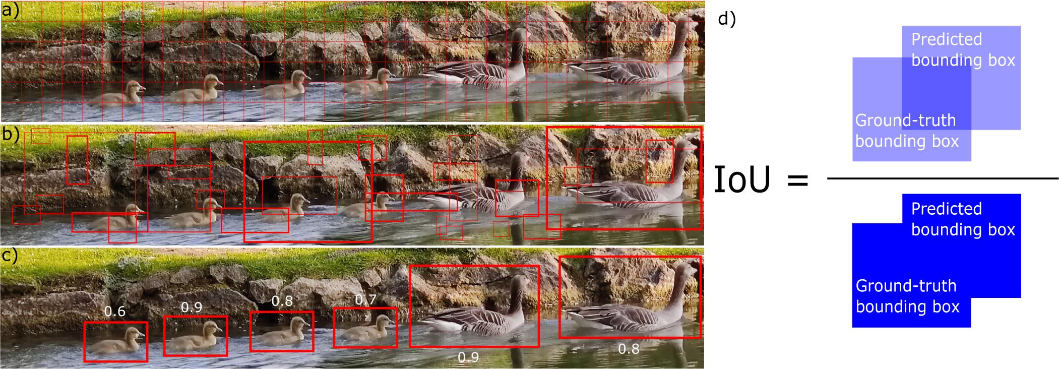
Fig. 1. Step-wise illustration of the object detection method. The example image presents ducks creating and surfing on wakefields. (a) Split the image into small grid cells; (b) predict bounding boxes and confidences for each class; (c) final detected objects with confidences; (d) bounding box predicted by the object detector versus the ground-truth bounding box labelled manually. IoU is defined as their area of intersection divided by their area of union, where an ideal object detector would have IoU = 1.

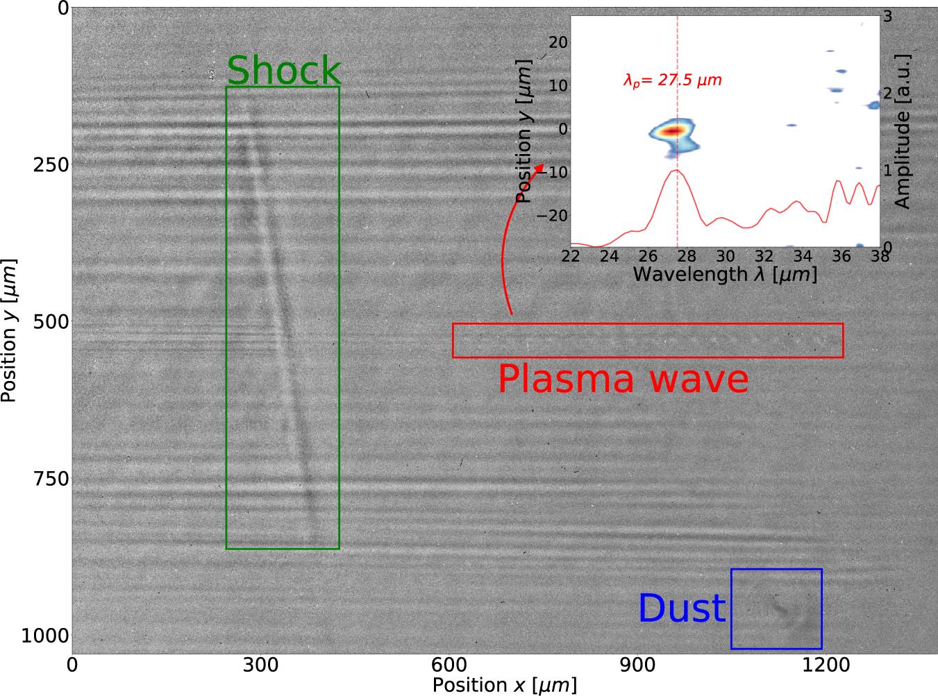
Fig. 2. An example: the plasma wave, the shock and the diffraction pattern caused by dust are found by the object detector and located with bounding boxes. More shadowgrams with different shock positions, without shocks, with multiple dust patterns and with overlapping objects are attached in the supplementary material. The subplot on the top right is the Fourier transform of the region within the bounding box of the plasma wave (red). The plasma oscillation wavelength is estimated by integrating along the vertical axis, which peaks at 27.5 μm.

Fig. 3. Plasma oscillation wavelengths (left-hand vertical axis) and plasma density (right-hand vertical axis) calculated from the Fourier transform results within the ROI defined by the object detector. (a) The backing pressure of the gas target is scanned from 1 to 6 bar. (b) The probe is moved from the upstream end to the centre of the gas target, and 0 mm is where the first plasma bubble of the plasma wave is at the density shock front. As mentioned in the main text, the region where the ROI includes the shock produces unreliable results and is thus greyed out.

Fig. 4. (a) Vertical position of the plasma wave moves over a day. (b) Jitter between every two consecutive shots, calibrated into a solid angle.

Fig. 5. Labelled peaks with charge number on electron energy spectra. The charge numbers are calculated from the integral within each bounding box.

Fig. 6. Detected interference pattern on a grating surface, originated from damages of previous optics in the amplification beam path: (a) is an image of the grating surface without damaged optics in the beam path, while (b) is an image of a grating surface with damaged optics in the beam path. The bounding boxes are drawn around the detected damage spots.

Table 1. Inference accuracy versus dataset size. The first column reports the size of the ground-truth (manually labelled) datasets for training, validation and testing. The second column reports the size of the augmented dataset for training, validation and testing. The third column presents the run time of the training process associated with each dataset, using a Tesla T4 GPU. The last two columns report the prediction accuracy of these datasets on two inference datasets, where inference set 1 has 50 images and inference set 2 has 1000 images.