
Jin Zhang, Yipeng Liao, Shiyuan Chen, Weixing Wang. Flotation Dosing State Recognition Based on Multiscale CNN Features and RAE-KELM[J]. Laser & Optoelectronics Progress, 2021, 58(12): 1215002
- Laser & Optoelectronics Progress
- Vol. 58, Issue 12, 1215002 (2021)
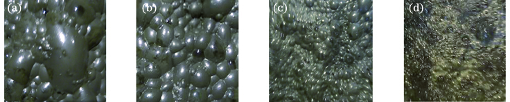
Fig. 1. Foam images in different dosing states. (a) s1; (b) s2; (c) s3; (d) s4
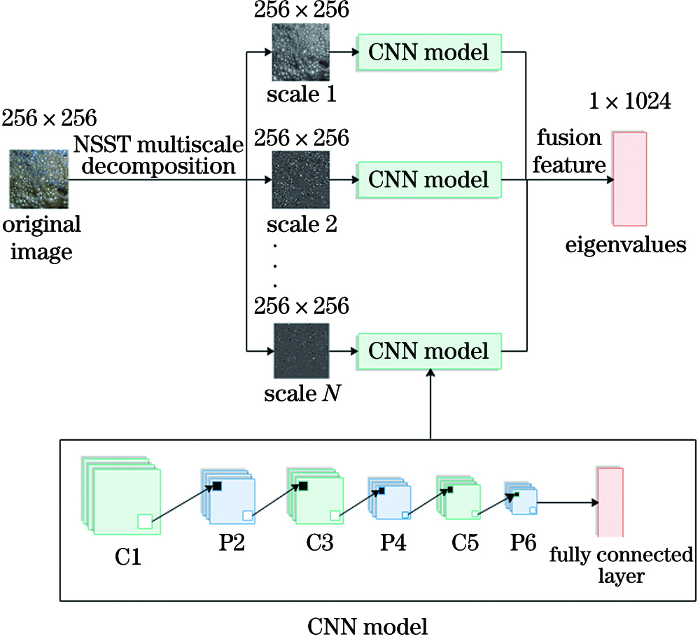
Fig. 2. Flow chart of the NSST-CNN model
Fig. 3. Structure of the RAE-KELM. (a) Self-encoder; (b) RAE-KELM
Fig. 4. Flow chart of the parameter optimization
Fig. 5. Overall framework of our method
Fig. 6. Performances of different optimization algorithms
Fig. 7. Visualization results of CNN features. (a) MNIST handwritten data set; (b) flotation foam image in state s1; (c) flotation foam image in state s2
Fig. 8. Testing accuracies of different feature extraction methods. (a) MNIST handwritten data set; (b) flotation foam image
Fig. 9. Recognition result of flotation dosing states
Fig. 10. Part of the recognized wrong image. (a) s1 is misjudged as s2; (b) s3 is misjudged as s2; (c) s4 is misjudged as s3
| |||||||||||||||||||||||||||||||||||||||||||||||||||||||||||||||||||||||||||||||||||||||||
Table 1. Parameters of the CNN model
| |||||||||||||||||||||||||||||||||||||||||||||||||||||||||||||||||||||||||||||||||||||||||||||||||||||||||||||||||||||||||||||||||||
Table 2. QBFA's average optimal value probability and number of iterations under different parameters
|
Table 3. Recognition results of flotation dosing states by different combination pairs
|
Table 4. Recognition results of different methods for flotation dosing states

Set citation alerts for the article
Please enter your email address
© Copyright 2018-2021 | Chinese Laser Press. All Rights Reserved 沪ICP备15018463号-20