Incompatibility of published ac magnetic susceptibility of a room temperature superconductor with measured raw data

J. E. Hirsch; D. van der Marel

doi:10.1063/5.0088429

Abstract

A material termed “carbonaceous sulfur hydride” has recently been reported to be a high-pressure room temperature superconductor [Snider et al., Nature 586, 373 (2020)]. We have previously pointed out that certain anomalies observed in the published data for the ac magnetic susceptibility of this material would be cleared up once the measured raw data were made available [J. E. Hirsch, arXiv:2110.12854v1 (2021) and J. E. Hirsch, Physica C 590, 1353964 (2021) (temporarily removed)]. The measured raw data, as well as numerical values of the data presented in figures in the aforementioned paper by Snider et al., have recently been posted on the arXiv [R. P. Dias and A. Salamat, arXiv:2111.15017v1 (2021) and R. P. Dias and A. Salamat, arXiv:2111.15017v2 (2021)]. Here, we report the results of our analysis of these raw data and published data and our conclusion that the raw data are incompatible with the published data. Implications of these results for the claim that the material is a room temperature superconductor are discussed.

I. INTRODUCTION

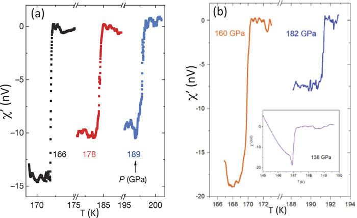
On October 14, 2020, Snider et al.1 reported the discovery of room temperature superconductivity in a material composed of hydrogen, sulfur, and carbon termed carbonaceous sulfur hydride, hereinafter called CSH. If this is true, it represents a major scientific breakthrough. “A superior test of superconductivity”1 demonstrating superconductivity was claimed to be the detection of sharp drops in the ac magnetic susceptibility. Figure 1 reproduces the results presented in Fig. 2a and Extended Data Fig. 7d of Ref. 1, showing susceptibility vs temperature for five different pressures, together with “raw data” in an inset for yet another value of the pressure. The five curves in Fig. 1 were obtained from the subtraction of two independent measurements, namely, “raw data” and “background signal,” according to the equation $data = raw data - background signal .$ (1)According to the caption of Fig. 2a of Ref. 1, “The background signal, determined from a non-superconducting C-S-H sample at 108 GPa, has been subtracted from the data.” Neither of these independent measurements (raw data and background signal) were given in the paper or in its supplemental material for the five pressures shown in Fig. 1. In a paper posted on the arXiv on December 1, 2021,2 the measured raw data for the three curves shown in Fig. 1(a) were made public by two of the authors of Ref. 1. In an update to Ref. 2 on December 28, 2021,3 the measured raw data and data for all the curves shown in Fig. 1 were made public.

Figure 1.Ac magnetic susceptibility of CSH at different pressure values reported in (a) Fig. 2a and (b) Extended Data Fig. 7d of Ref. 1. The inset in (b) shows “raw data” according to Ref. 1. Reprinted with permission from Snider et al., Nature 586, 373 (2020). Copyright 2020 Nature/Springer/Palgrave Nature.

Given the raw data and the data reported in Ref. 3, we can extract the background signal from the relation $background signal = raw data - data .$ (2)Figure 2 shows what the raw signal data given in Ref. 3 and the background signal resulting from Eq. (2) look like for the three curves shown in Fig. 1(a), without high resolution. The qualitative behavior is as expected: there are drops in the raw data superposed on an approximately linear background. Subtraction of the background gives the data in Fig. 1(a), where the drops become much more noticeable.

Figure 2.Raw data from Ref. 2 and background signal calculated from Eq. (2) for the data given in Fig. 1(a). In (a), the curves have been shifted horizontally and vertically so that they all fit on the same graph, without the scales being changed. In (b), the background signals obtained from Eq. (1) have been shifted vertically to get a smoothly varying slope. This is justified because the data shown in Fig. 1 have all been shifted vertically by an unknown amount so that they are all close to zero above the jump. The dashed lines in (b) have been inserted to guide the eye.

In Refs. 4 and 5, we suggested that various questions that we raised there and in an earlier paper6 about the validity of the magnetic susceptibility measurements reported in Ref. 1 would find answers once the authors of the latter released the underlying data. In this paper, we report our analysis of the data reported in Refs. 2 and 3 and our conclusion that the raw data underlying the published data are incompatible with the published data. Some of the results discussed here were presented earlier in a short communication7 and in preprints.8–10

II. RAW DATA AND BACKGROUND SIGNAL

Figures 3 and 4 show graphs of the susceptibility curves from Fig. 2a and Extended Data Fig. 7d of Ref. 1, respectively. The left panels show the curves with the same resolution as given in Ref. 1, and the right panels show the same curves with higher resolution.4

Figure 3.Magnetic susceptibility for pressures 166, 178, and 189 GPa of Fig. 2a of Ref. 1. The left panels show the curves with the same resolution as that in the figure published in Ref. 1, and the right panels show the same curves with higher resolution.

Figure 4.Magnetic susceptibility for pressures 160 and 182 GPa of Extended Data Fig. 7d of Ref. 1. The left panels show the curves with the same resolution as that in the figure published in Ref. 1, and the right panels show the same curves with higher resolution.

In Ref. 7, we plotted the background signal data obtained from Eq. (2) for all the temperature ranges where data and raw data have been reported, and we determined that it was impossible for the background signal to have resulted from a single measurement at 108 GPa, because the resulting function was double-valued in a certain temperature range. This already raises questions about how the background signal was obtained.

Figures 5–9 show the raw data from Ref. 3, the data published in Fig. 2a and Extended Data Fig. 7d of Ref. 1, and the background signal obtained from Eq. (2), for the five values of the pressure reported in Ref. 1, namely 166, 178, and 189 GPa in Fig. 2a of Ref. 1 and 160 and 182 GPa in Extended Data Fig. 7d. The scale on the vertical axis gives the susceptibility in nanovolts as given by the raw data of Ref. 3. The data curves (green curves) have been shifted vertically so that they coincide as closely as possible with the raw data curves. It can be seen that there is close agreement between the raw data (black points) and the data (green points) in the region where the raw data change rapidly with temperature. To facilitate comparison between raw data and background signal, a part of each background signal curve has been copied and shifted downward to be positioned near the raw data points.

Figure 5.For pressure 166 GPa, the black points are raw data from Ref. 3, the green curve is susceptibility data from Ref. 3, and the red points are background signal inferred from the raw data and published data according to Eq. (2). The lower part of the red curve has been duplicated and shifted down to facilitate comparison of the fine structure.

Figure 6.For pressure 178 GPa, the black points are raw data from Ref. 3, the green curve is susceptibility data from Ref. 3, and the red points are background signal inferred from the raw data and published data according to Eq. (2). The lower part of the red curve has been duplicated and shifted down to facilitate comparison of the fine structure.

Figure 7.For pressure 189 GPa, the black points are raw data from Ref. 3, the green curve is susceptibility data from Ref. 3, and the red points are background signal inferred from the raw data and published data according to Eq. (2). The lower part of the red curve has been duplicated and shifted down to facilitate comparison of the fine structure.

Figure 8.For pressure 160 GPa, the black points are raw data from Ref. 3, the green curve is susceptibility data from Ref. 3, and the red points are background signal inferred from the raw data and published data according to Eq. (2). The lower part of the red curve has been duplicated and shifted down to facilitate comparison of the fine structure.

Figure 9.For pressure 182 GPa, the black points are raw data from Ref. 3, the green curve is susceptibility data from Ref. 3, and the red points are background signal inferred from the raw data and published data according to Eq. (2). The lower part of the red curve has been duplicated and shifted down to facilitate comparison of the fine structure.

What should be apparent to the reader from looking at these figures is that the fine structure in the raw data (black points) and the background signal (red points) is nearly identical for all cases shown, and that that fine structure is absent in the data (green points). The only case where some of the fine structure in the raw data can be discerned in the data is for 182 GPa.

Is it possible that the coincidences seen in the fine structure of the raw data and inferred background signals in Figs. 5–9 may be real reproducible features associated with the measuring apparatus obtained in separate measurements at different pressures, as reported in Ref. 1? To assess this possibility, we present in Figs. 10 and 11 examples of susceptibility measurements in diamond anvil cells for other materials, where measurement results for overlapping ranges of temperature are shown. From a comparison of the regions highlighted by the rectangular boxes for curves at different pressures, it is apparent in Figs. 10 and 11 that the fine structure does change substantially with pressure in these type of measurements in diamond anvil cells. This indicates that it is impossible for the raw data and background signal to have the similar fine structure shown in Figs. 5–9 if they result from independent measurements.

Figure 10.Susceptibility measurements in diamond anvil cells for (a) yttrium under pressure, from Fig. 1 of Ref. 11 and (b) lead under pressure, from Fig. 3(a) of Ref. 12. Pressure values are given next to the curves. The rectangular boxes have been inserted to facilitate comparison of the fine structure of different curves in the same temperature range. (a) Reproduced with permission from Hamlin et al., Phys. Rev. B 73, 094522 (2006). Copyright 2006 the American Physical Society. (b) Reproduced from Feng et al., Rev. Sci. Instrum. 85, 033901 (2014) with the permission of AIP Publishing.

Figure 11.(a) Susceptibility measurements for (a) platinum hydride under pressure, from Fig. 2 of Ref. 13, (b) lithium metal under pressure, from Fig. 2 of Ref. 14, and (c) lutetium metal under pressure, from Fig. 4a of Ref. 15. The rectangular boxes have been inserted to facilitate comparison of the fine structure of different curves in the same temperature range. (a) Reproduced with permission from Matsuoka et al., Phys. Rev. B 99, 144511 (2019). Copyright 2019 the American Physical Society. (b) Reproduced with permission from S. Deemyad and J. S. Schilling, Phys. Rev. Lett. 91, 167001 (2003). Copyright 2003 the American Physical Society. (c) Reproduced with permission from Debessai et al., Phys. Rev. Lett. 102, 197002 (2009). Copyright 2009 the American Physical Society.

This then leads us to consider the following possible explanations for this conundrum:1.The raw data reported in Ref. 2 are not the raw data corresponding to the published data in Ref. 1. If that were to be the case, then our procedure for obtaining the background signal, Eq. (2), would be invalidated. However, the authors of Refs. 2 and 3 say that they are the same. In addition, it can be seen in Figs. 5–9 that in the regions of the transitions, there is a good coincidence between the published data (green curves) and raw data (black curves). Therefore, we have to discard this explanation.2.The published data in Ref. 1 resulted from a smoothing procedure performed on the difference between measured raw data and measured background signal that were independently noisy, which eliminated the fine structure. If so, then, in obtaining the background signal from the subtraction in Eq. (2), we would artificially introduce the fine structure of the raw data into the extracted background signal. However, it would not make sense to smooth the data to eliminate fine structure in the raw data of the magnitude shown in the figures and at the same time show fine structure in the data that are not contained in the raw data. To make this point even more clearly, we show in Fig. 12 raw data for small temperature intervals for pressures 166 and 189 GPa. The data for these regions were shown in Figs. 8 and 9 of Ref. 3. It can be seen in Fig. 12 that the variations with temperature observed in the green curves (data) are not contained in the raw data. Therefore, we have to discard this explanation.3.Either the raw data given in Refs. 2 and 3 or the published data in Refs. 1–3, or both, do not display the reality of what those papers say they display.

Figure 12.For small temperature intervals for pressures 166 and 189 GPa, respectively, (b) and (d) show data (green points), raw data (black points), and background signal (red points). (a) and (c) show the data with the vertical scale amplified to clearly reveal the fine structure.

To get an overview of the highly anomalous behavior of raw data and background signal discussed above, we plot the results for all pressures in Fig. 13. Note also the very different behavior of the raw data for 138 GPa compared with all other cases: only here does the slope of the raw data vs temperature change substantially right at the point where the drop in signal occurs. We discuss this further in Appendix A.

Figure 13.Comparison of fine structure in the raw data (black points) and background signal (red points). The lower red curves are identical to the upper red curves, shifted downward to facilitate comparison with the fine structure in the black curves for temperatures below the drops. The ordinate gives the voltage in nanovolts.

In the following sections, we will present a further analysis of these data, and in particular of the data for 160 GPa that show very anomalous features, which have been suggested to result from a particular background subtraction methodology termed “UDB_1” by the authors of Ref. 16. This will shed more light on the possible alternative explanations listed earlier in this section.

III. FURTHER ANALYSIS OF RAW DATA AND PUBLISHED DATA

From the analysis in Sec. II, we concluded that there is an unexpected disconnect between the published data for magnetic susceptibility in Ref. 1 and the raw data for the same measurements posted in Refs. 2 and 3. Our analysis in Sec. II relied on extracting the background signal. Here, we carry out a further comparison between raw data and published data without relying on an inferred background signal.

We consider the susceptibility increments $Δ χ_{i} \equiv χ_{i} - χ_{i - 1},$ (3)where χ_i is either the data or the raw data for point i. In the tables in Ref. 3, the data and raw data are all given for the same list of temperature values, which facilitates comparison. Figure 14 shows a comparison of the susceptibility increments for raw data and data for the six pressure values.

Figure 14.Comparison of susceptibility increments (in nV) for neighboring points in temperature between raw data (black points) and data (green points). All values have been obtained from the tables in Ref. 3.

Recall that an independently measured background signal is reportedly subtracted from the raw data to arrive at the published data [Eq. (1)]. However, Fig. 14 cannot be understood in light of Eq. (1). In particular, for 160, 166, 178, and 189 GPa, the range of values of Δχ for the raw data is much larger than the range of values of Δχ for the data. According to Eq. (1), we would expect exactly the opposite: given a range of values for Δχ for the raw data and another one for the independently measured background signal, the resulting range of values of Δχ for the difference, i.e., the data, should be larger than for both. Instead, it is substantially smaller.

The discrepancy between what we expect to see and what we see is particularly stark for 160 GPa. For that case, the Δχ increments for the data in Fig. 14 follow well-defined lines with no scatter at all. It is impossible to understand how this behavior can result from a physical measurement of a voltage and subtraction of a physical measurement of another voltage at a different pressure. In Fig. 15, we show in the left panel the susceptibility increments for the raw data (black points) and for the background signal obtained through Eq. (2) (red points). The difference between these two sets of points, obtained through what were said to be separate measurements at different pressures,1 which look highly random and uncorrelated, gives rise to the highly structured susceptibility increments for the data points shown in the right panel of Fig. 15.

Figure 15.For pressure 160 GPa, the left panel shows susceptibility increments for raw data (black points) and background signal obtained through Eq. (2) (red points). The right panel shows susceptibility increments for data, i.e., the difference between raw data and background signal shown in the left panel.

To further highlight the highly anomalous character of the data for 160 GPa, we show in Fig. 16 the data and raw data for limited ranges of temperatures below and above the steep drop in susceptibility. The raw data and background signal show large scatter and they track each other, as seen earlier in Fig. 8. The data, which result from subtracting the background signal from the raw data, follow a highly regular pattern, oblivious to the large oscillations in the raw data and background, with smooth connected pieces separated by discrete jumps. It is impossible to understand how such a pattern could result from any physical measurement vs temperature, or from a combination of physical measurements vs temperature. For the data (blue points) to result from subtraction of a background (red points) from raw data (black points), the oscillations in the background signal, presumably arising from instrumental noise, would have to closely track the oscillations in the raw data. Independently measured raw data and background signal do not have that property.

Figure 16.Raw data, data, and background signal inferred by subtraction, obtained from the numerical values reported in Table 5 of Ref. 3, for the low- and high-temperature regions of the 160 GPa data.

IV. DETAILED ANALYSIS OF 160 GPa DATA

Figure 17(a) shows the data on susceptibility for a pressure of 160 GPa. The numerical values are given in the second column of Table 5 of Ref. 3 (labeled “Superconducting Signal”). A superconducting transition appears to take place around T = 170 K. In Figs. 17(c) and 17(d), these data are shown on a 15-times expanded vertical axis. Because of the steep rise at 170 K the regions above and below 170 K need to be displayed in separate panels. A striking feature is the series of discontinuous steps. These steps are directly visible to the eye in the temperature ranges where χ′(T) has a weak temperature dependence. However, they are also present in the range where χ′(T) rises steeply as a function of temperature, as can be seen by calculating the difference between neighboring points $Δ χ (j) = χ (T_{j}) - χ (T_{j - 1}) .$ (4)This quantity, shown in Fig. 17(b), is the same as in the right panel of Fig. 15 except for the opposite sign, originating in the different definitions in Eqs. (3) and (4). It exhibits an intriguing “aliasing” effect in the “shadow curves” displaced vertically by integer multiples of 0.165 55. To make this crisp, the vertical axis of Fig. 17(b) corresponds to Δχ(j)/0.165 55. Clearly, this is a set of curves vertically offset by an integer n = −1, 0, 1, 2, 3, 4. The most systematic offsets in sign and size occur between 169.6 and 170.1 K.

Figure 17.(a) Susceptibility data (“Superconducting Signal”) for CSH at a pressure 160 GPa, from the numerical data of Table 5 of Ref. 3. (b) Difference between neighboring points of (a) divided by 0.165 55. (c) and (d) Data of (a) on an enlarged scale. (e)–(g) Data of panels (c), (d), and (a) after unwrapping with integer multiples of 0.165 55. The different colors in (e) and (f) refer to disconnected segments of (c) and (d). (h) Same as (b), but now using the unwrapped data of (g). The same vertical scale is used as in (b).

By shifting continuous segments of the curves by an amount 0.165 55n, with n integers that can be read off from Fig. 17(b), it is a simple and straightforward task to “unwrap” the vertical offsets. The result for the two separate ranges above and below 170 K is displayed in Figs. 17(e) and 17(f), and that for the full range is displayed in Fig. 17(g). On comparing Fig. 17(e) with Fig. 17(c), and Fig. 17(f) with Fig. 17(d), it is possible to verify that the resulting curves are extremely smooth and completely free of discontinuities. On comparing Fig. 17(g) with Fig. 17(a), it can be seen that the steep rise at 170 K is absent from Fig. 17(g). As a consistency check Δχ(j) was finally calculated, corresponding to Fig. 17(g). On comparing the result in Fig. 17(h) with that in Fig. 17(b) (shown with the same vertical scale to facilitate comparison), it can be seen that there are no shadow curves in Fig. 17(h), demonstrating that not only is the temperature dependence of Fig. 17(g) smooth, but the differential shown in Fig. 17(h) is, surprisingly for an experimental quantity, also completely smooth.

The behavior of the data shown in Figs. 17(c) and 17(d), together with the fact that the segments can be joined by vertical shifts that are all of the same form (0.165 55 ± 0.000 05)n, indicate that the disconnected segments are portions of a continuous curve that has been broken up by quantized steps. The sequence of steps together form a quantized component that is entirely responsible for the steep rise of χ′(T) at 170 K seen in Fig. 17(a). The data (Superconducting Signal) of Fig. 17(a) can be expressed as $\begin{align} Superconducting Signal & = quantized component \\ + unwrapped curve, \end{align}$ (5)where the unwrapped curve is given in Fig. 17(g). Figure 18 shows the same information as in Figs. 17(a)–17(d) for the quantized component. The connected segments are now horizontal, and the increments in Fig. 18(b) are integers.

Figure 18.(a) Quantized component of susceptibility data (“Superconducting Signal”) for CSH at a pressure 160 GPa. (b) Difference between neighboring points of (a) divided by 0.165 55. (c) and (d) Data of (a) on an enlarged scale.

According to Ref. 1, a background signal measured at 108 GPa was subtracted from the raw data (“Measured Voltage”) in obtaining the published data (“Superconducting Signal”) in Ref. 1. In other words, $Superconducting Signal = Measured Voltage - background signal$ (6)Comparison of Eqs. (6) and (5) strongly suggests that the Measured Voltage and background signal in Eq. (6) correspond to the quantized component and (−1) × unwrapped curve in Eq. (5), respectively.

A. A possible explanation of these results?

To begin to understand these results, we have to understand (a) why the Measured Voltage deduced above (quantized component) is a series of flat steps separated by jumps of a fixed magnitude 0.165 55 nV and (b) why the background signal deduced above (the negative of the unwrapped curve) is a smooth curve with no experimental noise.(a)A digital lock-in amplifier will yield discrete values for the measured voltages, where the size of the step between neighboring values of measured voltages is given by the instrumental resolution. Given our conclusion that the quantized component shown in Fig. 18(a) could be the raw data (Measured Voltage), this would indicate that the resolution of the instrument in this measurement was of order 0.2 nV. Such a low resolution could result from setting the digitizer range of the lock-in amplifier to a large value, ∼100 µV.¹⁷(b)The smooth behavior of the background signal [(−1) × Fig. 17(g)] could be explained if, rather than measured values of the background signal, a polynomial fit to the measured values were subtracted from the raw data. We note, however, that Ref. 1 does not mention such a procedure.

B. Relation with the reported raw data

In Sec. IV A, we have concluded that the very unusual nature of the susceptibility data for 160 GPa reported in Ref. 1 could possibly be understood if the measured raw data were the quantized component of the Superconducting Signal shown in Fig. 18(a), and the background signal were given by the negative of the unwrapped curve in Fig. 17(g). On the other hand, the superconducting signal as well as the measured raw data were reported in Table 5 of Ref. 3, and we can infer from them the background signal simply by subtraction. Therefore, in Figs. 19(a) and 19(b), we compare the reported raw data and the background signal inferred from the reported raw data and the reported data3 with our hypothesized raw data and background signal deduced above.

Figure 19.(a) Raw data (Measured Voltage) reported in Ref. 3 for 160 GPa (black points), compared with quantized component of susceptibility data (red points). (b) Background signal inferred by subtraction of reported raw data and data in Ref. 3 (black points), compared with background signal inferred from unwrapping of susceptibility data (red points).

It can be seen from Fig. 19 that there is a complete disconnect between the raw data and the background signal inferred from the numbers reported in Ref. 3, and the raw data and background signal inferred from the analysis of the Superconducting Signal1 (numerical values given in Ref. 3) discussed above. In particular, there is certainly no way that a polynomial fit of the black points in Fig. 19(b) would have any resemblance to the red curve shown in Fig. 19(b), and there is a significant difference between the black and red curves in Fig. 19(a). There is also no quantization of measured voltages in the raw data reported in Ref. 3. The reported measured values of the Measured Voltage are given in Table 5 of Ref. 3 with 11 significant digits. This is not necessarily the experimental resolution. The experimental resolution is set by the complete analog and digital chain, of which the digital-to-analog converter is the last element. The smallest step between neighboring temperatures in Table 5 of Ref. 3 is of order 0.0001 nV. Hence, the resolution of the experimental setup is 0.0001 nV or smaller. This is about three orders of magnitude higher resolution than the resolution of the measuring device that would yield the quantized component [red curve in Fig. 19(a)] as measured raw data. It can also be seen from Fig. 19 that there is much larger noise in the raw data and background signal reported in Ref. 3 than there is in the red curves that were deduced from the reported Superconducting Signal above. As discussed earlier, this is also found for all the other pressure values.

V. EXPLANATIONS BY THE AUTHORS OF REF. 1

It should be clear from the previous sections that there is an incompatibility between the statement in the original publication1 that the background signal was obtained from an independent measurement at a much lower pressure (108 GPa) and features seen in the raw data and the data. It turns out that in subsequent publications,3,16 the statement of Ref. 1 that “The background signal, determined from a non-superconducting C-S-H sample at 108 GPa, has been subtracted from the data” was explicitly (albeit unapologetically) negated by two of the authors of Ref. 1. We discuss this in what follows and in Appendix B.

In Refs. 2 and 3, the authors write

In the side-by-side coil magnetic susceptibility experiments, the large background signal is unique to each experiment, is temperature dependent, can have varying profiles, and a consequence of the makeup of both diamond anvil cells (DACs). However, the background can be approximated as linear in the region of the transition, and the susceptibility of the sample extracted after background subtraction. In the raw data a temperature region immediately above and below the transition is selected and a profile subtraction based on the similar temperature range from an additional measurement made at a nonsuperconducting pressure. The background profile is kept true but scaled to match the same signal strength of the desired measurement. This profile is then subtracted from the raw data, providing a baseline value of zero for the susceptibility above Tc.

The first part of this statement says that the background is approximated by a linear function fitted to match the slope of the measured raw data, and subtracted from the raw data. This is not the generally accepted procedure for performing background subtraction in these experiments, where the background is taken from an independent measurement.11–15 But it is at least an understandable statement and arguably a defensible procedure, provided it is clearly explained in the publication. However, in this case, we point out that (a) such a procedure was not discussed in the original publication1 and in fact contradicts what was stated there, namely, that the background was measured; and (b) such a procedure is not compatible with the behavior of the background signals seen in Figs. 5–9, which have the fine structure of the raw data.

The second part of the above quotation is not understandable, in particular the statement “The background profile is kept true but scaled to match the same signal strength of the desired measurement.” It is not clear what this statement means and how a reader can reproduce this “scaling,” since it is not explained, nor is any explanation given of the physical justification for this “scaling.” Furthermore it is stated that it relies on “a profile subtraction based on the similar temperature range from an additional measurement made at a nonsuperconducting pressure.” The authors have not released the underlying data of this “additional measurement made at a nonsuperconducting pressure,” despite repeated requests, nor have they described those measurements even qualitatively in any of their publications. Furthermore, this would not explain the similarity in the fine structure of raw data and background signal pointed out in earlier sections of the present paper.

Further explanations by the authors of Refs. 2 and 3 are given in Ref. 16, where they describe a method of background subtraction that they call “user defined background 1” (“UDB_1”). We discuss this in Appendix B.

VI. DISCUSSION

In the Fall of 2020, one of us (J.E.H.) requested the underlying data associated with the published susceptibility curves in Ref. 1 and asked for an explanation of the anomalous change in slope in the “raw data” susceptibility curve shown in the inset of Fig. 1.6 At the end of 2021, the requested data and explanation were posted on arXiv.2,3 Additional explanations for questions that we raised in a preprint posted in January 202218 were provided shortly thereafter in Ref. 16, which are discussed in Appendix B. Unfortunately, the information provided in those documents does not answer these questions; instead, it raises additional troubling ones.

In a nutshell, the key question addressed in this paper is whether the susceptibility data reported in Ref. 1 as evidence for room temperature superconductivity are supported by the underlying raw data reported in Ref. 3. The analysis in this paper leads to the unequivocal conclusion that the data reported in Ref. 1 could not have been obtained from the raw data reported in Ref. 3 using data analysis and processing consistent with standard scientific practice.

As discussed in Appendix A, no physical explanation was provided in Ref. 3 for the anomalous rise in χ below the jump in the raw data shown in the inset of Fig. 1 and noted in Refs. 4 and 6. None of the references cited in Ref. 3 (Refs. 20–22 in that paper) and claimed there to show such an anomalous rise do in fact show such behavior within a range of less than 2% of the presumed critical temperature as the inset of Fig. 1 shows, as readers can easily verify by reading those references. Nor has it been explained why the anomalous raw data of the inset of Fig. 1 were chosen to be shown in Ref. 1 instead of any of the typical raw data shown in Fig. 13 that do not show such an anomalous rise.

More troubling is the fact that the raw data provided in Refs. 2 and 3 that purportedly underlie the published susceptibility data in Ref. 1 exhibit a complete disconnect with the published curves they are supposed to represent. We have provided evidence that we regard as conclusive that the raw data presented in Refs. 2 and 3 cannot possibly give rise to the numerical values of the susceptibility provided in Refs. 2 and 3 and shown as curves in Ref. 1 without using procedures that can only be characterized as data alteration and manipulation, euphemistically called “user defined background method 1” in Ref. 16.

In particular, we have shown in Figs. 5–9 and 13 that fine structure in the raw data is closely reproduced in fine structure in the inferred background and is disconnected from fine structure contained in the data. These features are completely unexpected. Furthermore, Fig. 14 shows that there is a complete disconnect between the increments in temperature and susceptibility between neighboring points for raw data and published data for all pressure values. The increments in susceptibility for the raw data are approximately an order of magnitude larger than for the data. Additionally, we have called attention to the highly unusual features of the data for 160 GPa, which cannot be understood as arising from the measured raw data and any conceivable way to define a background that would be consistent with standard scientific practice.

The background subtraction method that was described in Ref. 1 was subsequently negated in Ref. 3 and again in Ref. 16, where yet other procedures were qualitatively described. None of those procedures were described in the original publication.1 In Appendix B, we point out that the “user defined background” procedure UDB_1 described in Ref. 16 is incompatible with generally accepted standard experimental practice. We also note that it took more than a year after the request4 for the raw data underlying the measurements reported in Ref. 1 for the authors of the latter to provide that information.

All of the above suggests consideration of the following equation that follows from Eq. (1) or Eq. (2):19 $raw data = data + background signal .$ (7)In other words, a physically reasonable approximately linear background signal with fine structure, as given by the red curves in Fig. 13, added to the data published in Fig. 2a and Extended data Fig. 7d of Ref. 1, would give rise to “raw data” identical to the black curves shown in Fig. 13, obtained from the columns labeled “Measured Voltage” of the tables in Refs. 2 and 3. It would of course be a misnomer to call such numbers obtained through Eq. (7) “raw data.”

In conclusion, we argue that we have shown in this paper that the ac magnetic susceptibility curves reported in Ref. 1 cannot have been obtained from the raw data published by two of the authors of Ref. 1 in Refs. 2 and 3 using procedures consistent with standard scientific practice. Consequently, those susceptibility curves provide no evidence for room temperature superconductivity of CSH,1 since they are unsupported by valid raw data. Why the authors of Refs. 2 and 3 present as raw data underlying the susceptibility curves of Ref. 1 values that are not consistent with the published data is an unanswered question.

ACKNOWLEDGMENTS

Acknowledgment. The authors are grateful to Kevin Smith, Samuel Weir, Alex Frano, Sunny Sinha, Annette Bussmann-Holder, Brad Ramshaw, and Peter Armitage for discussions and helpful input.

APPENDIX A: HISTORY AND REMARKS ON OTHER POINTS MADE IN REF. 2

Starting on November 12, 2020, one of us (J.E.H) attempted to obtain from the corresponding author and coauthors of Ref. 1 the raw data and background signal used to obtain the measurements shown in Fig. 1. Details of this saga are described in Refs. 4 and 5. Finally, on December 1, 2021, some of those data, namely, the measured raw data for the three curves shown in Fig. 1(a), as well as for the inset in Fig. 1(b), were made public in Ref. 2 by two of the authors of Ref. 1. On December 28, the measured raw data for the pressure curves shown in Fig. 1(b) were made available, as were all the numerical values of the data (“Superconducting Signal”) for all pressure values. The background signal data used, also requested more than a year ago, have not been made available, but can be obtained by subtracting data from raw data.

Figure 4 of Ref. 2, shown here as Fig. 20, compares the “raw data” for CSH shown in the inset of Fig. 1(b) with similar-looking data for the susceptibility of europium metal reported in Ref. 20. Such a comparison was made by us in Refs. 4 and 6. Reference 2 states “Remarkably, the measured signal strength is different in two samples, indicating different sample sizes.” Indeed, Fig. 20 shows a susceptibility jump of ∼−20 nV for CSH and −40 nV for Eu. It should be pointed out, however, that the susceptibility jump published in Ref. 20 for exactly the same case showed a jump of −20 nV and not −40 nV. Reference 2 makes the cryptic statement in the caption of their Fig. 4“Note that drop in signal in Eu is∼−40nV as observed before scaling due to different warming rates.” There is, however, no statement in Ref. 20 indicating that the warming rate would require scaling of the signal—quite the contrary, Ref. 20 only stated that “the observed Δχ′ ∼ 20nV jump atT_cis consistent with perfect diamagnetism, the hallmark of a superconductor.” There is also, to the best of our knowledge, no physical reason why the warming rate should cause a susceptibility drop due to onset of superconductivity to change by a factor of 2.

Figure 20.The curves shown in the figure were traced from the curves shown in Fig. 4 of Ref. 2. The figure caption in that paper reads “The AC susceptibility data of CSH at 138 GPa [1] and elemental Eu at 120 GPa from Debessai et al. [19]. Note that drop in signal in Eu is∼−40nV as observed before scaling due to different warming rates.”

Figure 21.The left panel shows susceptibility results presented in Fig. 2 of Ref. 20. The regions of the curve corresponding to 118 GPa enclosed in purple rectangles are shown enlarged in the right panel (with lower and higher temperature at the bottom and top, respectively). Note the identical patterns of both curves. Reproduced with permission from Matsuoka et al., Phys. Rev. B 99, 144511 (2019). Copyright 2019 the American Physical Society.

Figure 22.The curves shown here are the same as in Fig. 7 of Ref. 2, except that the black curve in the top panel is red in that figure and the red line in the top panel is black. The curves were generated using the data in the tables of Ref. 3. The labels next to the curves are the same as in Ref. 2. The caption of Fig. 7 of Ref. 2 reads “The AC susceptibility data from Snider et al., showing the raw data, the background used for subtraction and the data shown in the publication.”

Figure 23.Figure 2 of Ref. 16, redrawn by us using the data in the tables of Ref. 3. We reproduce the caption given in Ref. 16 here: “AC susceptibility data. (a) Raw data measured at 160 GPa. The profile of the regions highlighted in blue are used as part of the UDB_1. (b) Measured voltage from the susceptibility measurement explained in experimental details section in Refs. 1 and 2 for 160 GPa. Raw data (red), UDB_1 (blue) and raw data−UDB_1 (black).” (Note that Refs. 1 and 2 in that text are Refs. 1 and 3 in the present paper.

So, according to Ref. 2, the top black curve of Fig. 22 is “raw data,” the red straight line is “background,” and the bottom curve is “data” as given by Eq. (1). It remains a puzzle why both curves show a large change in slope between above and below T_c, an anomaly first noted in Refs. 4 and 6. It is also perplexing that the lower “data” curve in Fig. 22 looks qualitatively different from the other five “data” curves for susceptibility shown in Fig. 1 that reportedly also had background subtracted.

Note also in Fig. 13 that the raw data for all pressures other than 138 GPa have a qualitative feature different from those at 138 GPa: their slopes are approximately the same before and after the drop interpreted as onset of superconductivity. Given those “typical” raw data, it is incomprehensible that the authors of Ref. 1 would have chosen to present there the highly atypical “raw data” or “data” for 138 GPa shown in the inset of Fig. 1.

Furthermore, Ref. 2 shows in its Fig. 5 a curve for “AC susceptibility of a sample which superconducts at 235 K” that shows a drop in susceptibility of ∼60 nV, which is four to eight times larger than the drops reported by the authors earlier¹ and shown in Fig. 1 of the present paper. Since the magnitude of the jump attributed to superconductivity is supposed to be proportional to the volume of the sample,¹⁵ this is perplexing given that Ref. 2 does not say that a much larger sample was used in that case.

In summary, no physical explanation for the large change in slope from above to below the jump in susceptibility shown in the inset of Fig. 1, i.e., the anomalous behavior that raised our concern with these measurements originally,⁶ has ever been provided.

APPENDIX B: FURTHER EXPLANATIONS BY THE AUTHORS OF REF. 3 GIVEN IN REF. 16

We turn now to Ref. 16, where further new descriptions of the process of background subtraction used were provided. Figure 23 shows Fig. 2 of that paper, for 160 GPa, redrawn by us using the data in the tables of Ref. 3 because we were not granted permission by the authors of Ref. 16 to reproduce it from their paper. The first part of the text in Ref. 16 associated with it reads as follows [where Ref. (2) is Ref. 3 of the present paper, and Figs. 2a and 2b are the left and right panels of the present Fig. 23]:

We once again emphasize the method of selecting the background as we described in the Ref. (2). In the side-by-side coil magnetic susceptibility experiments, the large background signal is unique to each experiment, is temperature dependent, can have varying profiles, and is a consequence of the makeup of the DAC (diamond anvil cell). However, the background can be approximated as linear in the region of the transition, and the susceptibility of the sample extracted after the background signal is subtracted from the raw data (as shown in Fig. 2a). We described this in more detail by looking at the AC susceptibility data for CSH at 138 GPa in Ref. 2. In the raw data a temperature region immediately above and below the transition is selected (as highlighted in blue and shown in Fig. 2b). The background profile is kept true but scaled to match the same signal strength of the raw data. This background profile is then subtracted from the raw data, providing a baseline value of zero for the susceptibility aboveT_c(as shown in Fig. 2b).

The first part of this statement appears to say that the background is approximated as linear. However, the background shown in the right panel of Fig. 23, labeled “UDB_1,” is not a linear function but has oscillations. Once again, the statement “The background profile is kept true but scaled to match the same signal strength of the raw data” is not explained and hence cannot be understood.

In their next paragraph, the authors of Ref. 16 expand on the meaning of their Fig. 2 (Fig. 23 here). We reproduce the paragraph in full below [where “Hirsch and van der Marel …arXiv. (3)” refers to an earlier version of Ref. 10, namely, Ref. 18]:

We further describe the user defined background. The background arises from fluctuating currents in the normal sample and the surrounding metals such as the gasket and cell; these give rise to a voltage in the pickup coil. We selected the background after carefully investigating the temperature dependence of the non-superconducting CSH sample at 108 GPa, the closest pressure prior to the superconducting transition. We note here that we did not use the measured voltage values of 108 GPa as the background. We use the temperature dependence of the measured voltage above and below theT_cof each pressure measurement and scale to determine a user defined background (Fig. 2a). The scaling is such that one achieves an approximately zero signal above the transition temperature; the subtracted background isolates the signal due to the sample. We call this method “user defined background method 1 (UDB_1)” in this report. With UDB_1, one finds a signal as a function of temperature comparable to what one observes on a large sample where the background is insignificant. This procedure is either not understood or intentionally ignored by Hirsch and van der Marel in their recent comments on the arXiv. (3) In other words, the background is not an independently measured signal as Hirsch and van der Marel incorrectly claim. See Fig. 2. We chose the UDB_1 background as opposed to a simple linear function, which we examine later, to make sure we captured the response of the unknown background contributions. Furthermore, the temperature vs time profiles are extremely difficult to accurately replicate between runs and hence why we use the profiles from the same dataset, before and after the superconducting transition to generate a user defined background profile. We will show that the function of the background, although subtly affects the signal to noise, does not detract from the clear presence of the raw, measured susceptibility response of the superconducting transition that clearly matches the independent electrical transport measurements. The user defined background for subtraction is qualitative in nature and does not represent a physical quantity, and we will demonstrate other methods later in this paper.

First, it is stated that “We selected the background after carefully investigating the temperature dependence of the non-superconducting CSH sample at 108 GPa, the closest pressure prior to the superconducting transition,” yet immediately thereafter it is stated that “We note here that we did not use the measured voltage values of 108 GPa as the background,” thus contradicting the immediately preceding statement as well as statements in both Refs. 1 and 3 in one fell swoop. Instead, the authors state that they used the measurements made at the same pressure (i.e., the raw data) to determine a “user defined background,” which they term “UDB_1.” They state that they “scale” it, but do not explain how. They state that they do not use a simple linear function, in contradiction to the statement in Ref. 3. Finally, they state “The user defined background for subtraction is qualitative in nature and does not represent a physical quantity.”

It is not standard scientific practice to use as “background” the same data as the raw data from which the background is to be subtracted. Furthermore, these statements do not explain how the background UDB_1 is actually chosen. It can be seen in the right panel of Fig. 23 that the background has the same “wiggles” as the raw data, as we have already pointed out in Fig. 8 for this pressure. If this background were chosen by taking “the profiles from the same dataset,” perhaps shifting uniformly and/or scaling uniformly, then, upon subtracting it from the raw data, one should obtain simply a constant for the data in that temperature range, or possibly a function that mirrors the fine structure of the raw data. Neither of those occurs for the data (black curve in the right panel of Fig. 23) that has its own independent wiggles, nor for other pressures. Furthermore, it should be recalled from the preceding sections that the data for 160 GPa exhibit highly structured and unusual behavior (see, e.g., Fig. 16) that in no way can be associated with anything stated by the authors of Ref. 16 in the paragraph quoted above.

In other parts of Ref. 16, the authors discuss other background subtraction methods (termed “UDB_2” and “UDB_3”), using linear functions. However, these are not applicable to any of the results for the five pressure values shown in Figs. 5–9. Therefore, we have to conclude that the same UDB_1 method was used for all the pressure curves published in Ref. 1. No further explanation about UDB_1 is given in Ref. 16 or in any other papers.

It should also be emphasized that the authors of Ref. 16 have not provided a clearly defined procedure for UDB_1 by which a reader can use the numerical values of the raw data and other information supplied by the authors except the data themselves and following that procedure obtain the background data used and the data reported. They have not given a hint of an explanation for how the highly structured 160 GPa data would result from the noisy 160 GPa raw data.

In summary, the mysterious UDB_1, “user defined background method 1,” cannot explain the disconnect between raw data and data pointed out in the preceding sections, and it cannot explain the highly unusual features of the data for 160 GPa shown in Figs. 15 and 16, or certainly the fact that the data can be decomposed as the sum of a quantized component plus a smooth continuous “unwrapped” curve as shown in Fig. 17.

In Appendix C, we address the arguments presented in Ref. 16 that “the analysis by Hirsch and van der Marel is non-scientifically based.”

APPENDIX C: DETAILED RESPONSE TO REF. 16

Here we address the discussion by Dias and Salamat (hereinafter DS) in Ref. 16, where they argue that “the analysis by Hirsch and van der Marel is non-scientifically based,” in reference to our preprint Ref. 18.

In Ref. 16, DS say that we constructed what we call the “quantized component” through a “nonscientific way,” as $F (j) = [χ (j - 1) - χ (j)] / 0.1655$ (C1)and then “rounded” F(j) to the nearest integer. They claim that they carried out the same steps and reproduced 97.77% of our values, and they explain the discrepancy by stating that we “handpicked” the remaining 2.23%. They also call 0.1655 an “arbitrary factor.”

Figure 24 shows the same content as Fig. 9 of Ref. 16. The black line is the susceptibility data for 160 GPa (top panels of Fig. 4 in the present paper). The green curve is what is obtained using DS’s “rounding off” procedure, and the blue curve close to it is what we obtained as the “unwrapped curve” [i.e., Fig. 17(g) in the present paper]. The magenta curve is what DS obtained as the “quantized component” with their rounding off procedure, and the red curve next to it is what we obtained [i.e., the negative of Fig. 18(a) in the present paper]. The fact that Fig. 24 is identical to Fig. 9 of Ref. 16 shows that we understand the procedure that DS used, and why they misunderstood what our paper¹⁸ says.

Figure 24.The content of Fig. 9 of Ref. 16, redrawn by us. The black curve shows the susceptibility data for 160 GPa. The green and magenta curves show the “unwrapped curve” and “quantized component” following the procedure described in Ref. 16. The dark blue and red curves show the corresponding quantities in our procedure. The figure is identical to Fig. 9 of Ref. 16.

Figure 25.Unwrapped curve and its derivative obtained with the rounding-off procedure of Ref. 16. Note the discontinuities in the slope, encircled in red.

Figure 26.First derivative of the unwrapped curve using as “arbitrary factor” 0.18 instead of 0.165 55.

In conclusion, the statements in Ref. 16 that “Hirsch and van der Marel changed this value by hand by looking at the artifacts ofF(j) in a non-scientific way,” that “They handpick values for temperatures between 172.2331 and 172.1116 K,” that 0.165 55 is an “arbitrary factor,” that “the analysis by Hirsch and van der Marel is non-scientifically based,” and that the “authors of Ref. (3) misled the scientific community” are all incorrect and a consequence of misunderstanding of our paper.¹⁸ The fact is, we have shown that there is a unique way to decompose the reported “data” for 160 GPa as the sum of a continuous curve with continuous derivatives and a discrete curve with values 0.165 55n, and that these components bear no resemblance to the “Measured Voltage” and inferred background signal reported in Ref. 3.

References

[1] E.Snideret?al.. Room-temperature superconductivity in a carbonaceous sulfur hydride. Nature, 586, 373(2020).

[2] R. P.Dias, A.Salamat. Standard superconductivity in carbonaceous sulfur hydride(2021).

[3] R. P.Dias, A.Salamat. Standard superconductivity in carbonaceous sulfur hydride(2021).

[4] J. E.Hirsch. On the ac magnetic susceptibility of a room temperature superconductor: Anatomy of a probable scientific fraud(2021).

[5] J. E.Hirsch. Physica C, 590, 1353964(2021).

[6] J. E.Hirsch. About the pressure-induced superconducting state of europium metal at low temperatures. Physica C, 583, 1353805(2021).

[7] J. E.Hirsch. Comment on ‘Room-temperature superconductivity in a carbonaceous sulfur hydride’ by Elliot Snider et al.. Europhys. Lett., 137, 36001(2022).

[8] J. E.Hirsch. Disconnect between published ac magnetic susceptibility of a room temperature superconductor and measured raw data. Preprints, 2021, 2021120115.

[9] J. E.Hirsch. Incompatibility of published ac magnetic susceptibility of a room temperature superconductor with measured raw data. Preprints, 2021, 2021120188.

[10] J. E.Hirsch, D.van der Marel. Extended Comment on Nature 586, 373 (2020) by E. Snider et al.

[11] J. J.Hamlin, J. S.Schilling, V. G.Tissen. Superconductivity at 17 K in yttrium metal under nearly hydrostatic pressures up to 89 GPa. Phys. Rev. B, 73, 094522(2006).

[12] Y.Feng, T. F.Rosenbaum, D. M.Silevitch. A compact bellows-driven diamond anvil cell for high-pressure, low-temperature magnetic measurements. Rev. Sci. Instrum., 85, 033901(2014).

[13] T.Matsuokaet?al.. Superconductivity of platinum hydride. Phys. Rev. B, 99, 144511(2019).

[14] S.Deemyad, J. S.Schilling. Superconducting phase diagram of Li metal in nearly hydrostatic pressures up to 67 GPa. Phys. Rev. Lett., 91, 167001(2003).

[15] M.Debessai, J. J.Hamlin, J. S.Schilling. Comparison of the pressure dependences of T_c in the trivalent d-electron superconductors Sc, Y, La, and Lu up to megabar pressures. Phys. Rev. B, 78, 064519(2008).

[16] R. P.Dias, A.Salamat. Reply to ‘Comment on Nature 586, 373 (2020) by E. Snider et al.(2022).

[17] B.Ramshaw(2022).

[18] J. E.Hirsch, D.van der Marel. Comment on Nature 586, 373 (2020) by E. Snider et al.

[19] This equation was previously conjectured in Ref. 8 from the fact that the noise in the data is significantly smaller than in the raw data.

[20] M.Debessai, J. J.Hamlin, T.Matsuoka, J. S.Schilling, K.Shimizu. Pressure-induced superconducting state of europium metal at low temperatures. Phys. Rev. Lett., 102, 197002(2009).

[21] M.Debessai, J. J.Hamlin, T.Matsuoka, J. S.Schilling, K.Shimizu. Retraction: Pressure-induced superconducting state of europium metal at low temperatures [Phys. Rev. Lett. 102, 197002 (2009)]. Phys. Rev. Lett., 127, 269902(2021).

微信扫一扫：分享

微信扫一扫：分享