Optical coherence state is one of the intrinsic characteristics of a partially coherent beam (PCB), describing the electric field correlation at pairs of spatial locations and times¹. In the space-frequency domain, spatial coherence properties are characterized by the two-point spectral degree of coherence (DOC) function, being a normalized version of the cross-spectral density (CSD) function. Over past several decades, the PCBs have attracted substantial academic attention owing to their capability to resist turbulence-induced negative effects and to reduce the speckle noise, and therefore, they have found important applications in free-space optical communications, laser materials processing, inertial confinement fusion, optical imaging, etc.^1-6. The Schell-model beams whose DOC is only a function of the separation of two spatial points are the most commonly encountered PCBs. They were extensively studied in the past few decades. However, these studies were mainly limited to Gaussian Schell-model beams, i.e., those with the DOC having a Gaussian profile. One of the difficulties for constructing a physically reliable PCB with non-Gaussian, and more generally non-Schell-like correlations, is that the CSD function must satisfy some constraints such as Hermiticity and non-negative definiteness. In 2007, Gori and co-workers applied the Bochner theorem of functional analysis for suggesting a sufficient and necessary condition to devise genuine CSD functions⁷ (see ref.⁸ for its vectorial generalization). Since then, the extensive work has been devoted to devising PCBs with different kinds of DOCs^9-11, propagation characteristics and interaction with matter^12-20. In particular, it was established that the DOC can be used as a new degree of freedom to control the free-space beam evolution and its interactions with linear media to reduce the turbulence-induced effects, and so on. Consequently, the PCBs with the prescribed DOC have recently become promising candidates in diverse applications including self-reconstruction, super resolution imaging, diffractive imaging and optical encryption^21-29. However, the DOC is not propagation-invariant which hinders its use in technologies requiring optical information transfer and recovery. The general problem of modeling of the PCBs whose DOC remains propagation invariant has not yet been tackled.

High-resolution image recovery is a complex problem that has been classically approached by means of the optical signal’s average intensity manipulations³⁰. In general, amplitude, phase, polarization, spectrum and other parameters of the wave-field are available for imaging or image acquisition^25-34. Nevertheless, in some practical situations such as in the presence of turbulence or turbidity, the amplitude and phase are susceptible to the influence of turbulence³⁵. The image information contained in the amplitude or in the phase becomes lost with propagation range. Hence, one has to explore other parameters for transmitting/retrieving image information. In fact, it was shown in recent studies^36-38 that the modulus of the DOC of the field scattered from a turbid medium is an efficient parameter that can be used to retrieve the embedded object’s information. However, since the DOC changes on propagation, it appears to be applicable only for short-distance image reconstruction.

In this article, we report that in situations when a cross phase (CP) is imposed on a PCB, the far-field modulus of its DOC propagating through free space, a paraxial optical system, and atmospheric turbulence returns to its value in the source plane. This finding is demonstrated through numerical examples and experiments. Further, based on the peculiar recovery feature of the DOC, an efficient approach is proposed for encoding the image information into the DOC profile and its transmission through both free space and atmospheric turbulence. The obtained image is, indeed, shown to be resistant to the negative effects induced by turbulence. This paper is organized as follows. First, the effect of the CP on the DOC of a PCB during propagation is studied theoretically. Next, the experiment is carried out to demonstrate the recovery of the far-field DOC in free space and in atmospheric turbulence. Then, a new scheme for the transmission of image via the DOC through the free space and turbulence is studied and the robustness of far-field imaging is demonstrated. Finally, the results are summarized.

Suppose a scalar, quasi-monochromatic Schell-model beam carrying a CP, propagates along the z-axis. In the source plane (z=0), the CSD function of such a beam has the following form¹²

${W_0}\left( {{{\boldsymbol{r}}_1},{{\boldsymbol{r}}_2}} \right) = \tau \left( {{{\boldsymbol{r}}_1}} \right){\tau ^*}\left( {{{\boldsymbol{r}}_2}} \right){\mu _0}\left( {\Delta {\boldsymbol{r}}} \right){\rm{exp}} \left[ {{\rm{i}}u\left( {{x_1}{y_1} - {x_2}{y_2}} \right)} \right]\;,$ (1)

where r_i =(x_i, y_i), i=1, 2 denote two arbitrary transverse position vectors, perpendicular to the z-axis; ∆r=r₁−r₂=(∆x, ∆y) is the difference of two position vectors and τ(r) is a complex amplitude function. For simplicity, we assume that the amplitude function is Gaussian: τ(r)=exp(−r²/4ω₀²) with ω₀ being the beam width while μ₀(∆r) is the DOC, which only depends on the difference of r₁ and r₂. The last term exp[iu(x₁y₁−x₂y₂)] is the CP, where u is a measure of the strength of the CP. The sign of the parameter u only determines the rotation direction of the beam³⁹. It can be regarded as the extension of astigmatic phase, and it is a separable function with respect to (x₁, y₁) and (x₂, y₂). Due to the coupling of the x and y in the CP, the beam will exhibit the particular distribution orbital angular momentum (OAM) flux density along the propagation direction, which is responsible for the rotation of beam spot during propagation. The CP has been extensively explored^39-44. The studies reveal that such a phase structure can make the beam rotate³⁹, realize coherent modes conversion⁴¹, flexibly focus the ring Pearcey beam⁴², as well as manipulate the high-order optical vortices^{43, 44}.

In order to investigate the effect of the CP on the evolution of the DOC, we first set μ₀(∆r) as the cosine-Gaussian correlated Schell-model (CGCSM) source¹⁶

$\;{\mu _0}\left( {\rm{\Delta}}{ {\boldsymbol{r}}} \right) = \cos \left( {\frac{{n\sqrt {2\pi } \Delta x}}{{{{i\text{δ}} _0}}}} \right)\cos \left( {\frac{{n\sqrt {2\pi } \Delta y}}{{{{i\text{δ}}_0}}}} \right)\exp \left({ - \frac{{\Delta {{\boldsymbol{r}}^2}}}{{2{i\text{δ}}_0^2}}} \right)\;,$ (2)

where δ₀ denotes the source coherence width and n is the beam order. Within the regime of paraxial approximation, the relationship between the CSD function in the source plane and the receiver plane containing a generic paraxial ABCD optical system is given by the Collins formula¹⁴

$$$\begin{array}{rl}& W\left({\text{boldsymbol}\mathit{\text{ρ}}}_1,{\text{boldsymbol}\mathit{\text{ρ}}}_2\right)=\frac{k^2}{4{\pi }^2{\text{boldsymbol}B}^2}\mathrm{e}\mathrm{x}\mathrm{p}\left[-\frac{\mathrm{i}k\text{boldsymbol}D}{2\text{boldsymbol}B}\left({\text{boldsymbol}\mathit{\text{ρ}}}_1^2-{\text{boldsymbol}\mathit{\text{ρ}}}_2^2\right)\right]\\ & \times {\int }_{-\mathrm{\infty }}^{\mathrm{\infty }}{\int }_{-\mathrm{\infty }}^{\mathrm{\infty }}{W}_0\left({\text{boldsymbol}r}_1,{\text{boldsymbol}r}_2\right)\mathrm{e}\mathrm{x}\mathrm{p}\left[-\frac{\mathrm{i}k\text{boldsymbol}A}{2\text{boldsymbol}B}\left({\text{boldsymbol}r}_1^2-{\text{boldsymbol}r}_2^2\right)\right]\\ & \times \mathrm{e}\mathrm{x}\mathrm{p}\left[\frac{\mathrm{i}k}{\text{boldsymbol}B}\left({\text{boldsymbol}r}_1\cdot {\text{boldsymbol}\mathit{\text{ρ}}}_1-{\text{boldsymbol}r}_2\cdot {\text{boldsymbol}\mathit{\text{ρ}}}_{\mathbf{2}}\right)\right]{\mathrm{d}}^2{\text{boldsymbol}r}_1{\mathrm{d}}^2{\text{boldsymbol}r}_2,\end{array}$$$ (3)

where k = 2π/λ stands for the wavenumber with wavelength λ, ρ₁ and ρ₂ denote two transverse position vectors in the receiver plane, and A, B and D are the elements of the optical system’s transfer matrix. Let us consider a single-lens focusing system: a thin lens with focal length f is placed in the source plane followed by free-space path of distance z after the lens. Under this circumstance, the elements of the transfer matrix are found from the ABCD matrix multiplication as

$\left( {$$\begin{array}{cc}\text{boldsymbol}A& \text{boldsymbol}B\\ \text{boldsymbol}C& \text{boldsymbol}D\end{array}$$} \right) = \left( {$$\begin{array}{cc}1& z\\ 0& 1\end{array}$$} \right)\left( {$$\begin{array}{cc}1& 0\\ -1/f& 1\end{array}$$} \right) = \left( {$$\begin{array}{cc}1-z/f& z\\ -1/f& 1\end{array}$$} \right)\;.$ (4)

On substituting Eqs. (1), (2) and (4) into Eq. (3) and after integration, we obtain the analytical expression for the CSD function in the receiver plane (see supplementary material). Interestingly, it is found that in the focal plane (z = f, namely, in the far field), the modulus of the DOC reduces to the following form

$\left| {{\mu _f}\left( {{\rm{\Delta}} {\boldsymbol{\textit{ρ}}} } \right)} \right| = \left| {\cos \left( {\frac{{n\sqrt {2\pi } \Delta {ρ _x}}}{{{{i\text{δ}} _f}}}} \right)\cos \left( {\frac{{n\sqrt {2\pi } \Delta {{ρ} _y}}}{{{{i\text{δ}} _f}}}} \right)\exp \left( { - \frac{{\Delta {\boldsymbol{\textit{ρ}}} _{}^2}}{{2{i\text{δ}} _f^2}}} \right)}\right|\;,$ (5)

where δ_f = (fu/k)δ₀ is the coherence width in the focal plane and ∆ρ = ρ₁−ρ₂ = (∆ρ_x, ∆ρ_y), provided that factor u satisfies condition

$ u>{\rm{max}}\left\{\sqrt{\rm{400}\pi {n}^{\rm{2}}/{{i\text{δ}} }_{0}^{2}-{\Omega }^{2}}/{\omega }_{0}, \sqrt{10}\Omega /\omega_{0}\right\}\;,$ (6)

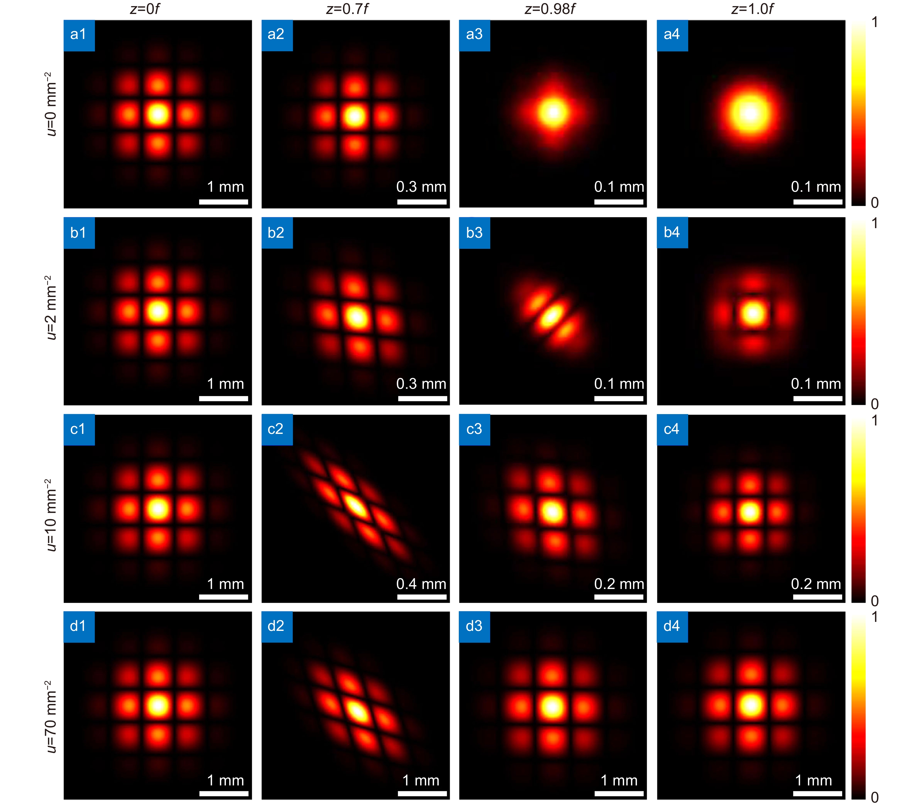
where Ω²=1/4ω₀²+1/δ₀². On comparing Eq. (5) to Eq. (2), we establish that the modulus of the DOC in the focal plane has the same form as that in the source plane but a different value of the coherence width. This peculiar propagation feature is quite different from that of the CGCSM beam without the CP, whose DOC in the focal plane degenerates to other forms. In general, the DOC itself can be complex already at the source plane due to the effects of the initial CP, and/or may become even more complex during propagation. Nevertheless, the modulus of the DOC in the focal region returns to the same form as it is in the source plane. In Fig. 1 the evolution of |μ| with propagation distance z, for different strength factors is presented. The first row is set for comparison, for the case of trivial CP, i.e., u = 0. In the absence of CP or when factor u is small (u = 2 mm⁻²), the modulus of the DOC gradually transforms to other shapes near the focal region [see first and second rows]. As the value of strength factor reaches 10 mm⁻² or higher [while satisfying Eq. (6)], it can be seen that the modulus of the DOC near the focal plane indeed returns to that in the source plane. Note that the DOC is twisted and rotates during propagation because of the CP’s presence [see Fig. 1(c2) and 1(d2)]. In fact, the DOC in the focal plane rotates π/2 rad, but its shape is unchanged. The rotation of the DOC attributes to the particular orbital angular momentum (OAM) flux density induced by the CP³⁹.

Although in the preceding analysis, a specific example is used for μ₀(∆r), the discovered phenomenon of the recovery of the DOC’s modulus in the focal plane (far field) can be generalized to any Schell-model beam carrying the CP. To justify this claim, a rather general alternative form of the DOC representing the Fourier transform of letter “S” (known as the power spectral density) is chosen as the example, [see the top right corner of Fig. 2(a)]. In this case, the DOC is a complex-valued function not assuming any analytical expression. The numerical result for the modulus of the DOC in the source plane is shown in Fig. 2(a). When such a beam carrying a CP with strength factor u=−60 mm⁻² propagates through the focusing system, the modulus of the DOC distribution undergoes shaping and rotating [see in Fig. 2(b) and 2(c)]. It gradually turns back to the initial form, with the expected 90-degree pattern rotation [see in Fig. 2(d)] in the focal plane. The examples based on other Schell-model sources carrying the CP (not shown here) also confirm this far-field DOC’s modulus recovery mechanism. In addition, the focusing lens does not need to be placed in the source plane of the beam. In fact, it can be placed in any transverse propagation plane z = const. And in the focal plane of the lens, the modulus of the DOC is also the same as that in the source plane (z = 0), irrespective of the DOC distribution at the plane where the focusing lens is placed.

In this section, we carry out the experiment to demonstrate the results obtained in the previous section. Figure 3 illustrates the schematic diagram for the experimental setup. It includes three parts. Part I is the optical system for the generation of a Schell-model beam with a CP. A laser beam emitted from a Nd:YAG laser (λ = 532 nm) is reflected by a mirror and expanded by a beam expander (BE), then arrives at a spatial light modulator (SLM₁). A computer-generated hologram is loaded on the SLM₁ which is used to produce a prescribed intensity pattern on the front surface of a Rotating Ground Glass Disk (RGGD). The scattered light is then collimated by a Lens L₁ and is transformed from the uniform light intensity to a Gaussian distribution by a Gaussian amplitude filter (GAF). If the size of the intensity pattern on the RGGD is much larger than the inhomogeneity scale of the RGGD, the DOC of the beam in the GAF plane can be described as the following integral according to the Van-Cittert Zernike theorem¹

$\mu ({\rm{\Delta}} {\boldsymbol{r}}) \propto \int {P({\boldsymbol{v}}){\rm{exp}} ( - {\rm{i}}2{\rm{\pi}} {\boldsymbol{v}} \cdot {\rm{\Delta}} {\boldsymbol{r}}/\lambda f){{\rm{d}}^2}{\boldsymbol{v}}}\; ,$ (7)

where P(v) is the intensity distribution in the RGGD plane, also known as the power spectral density in the literatures^15-17. The generated partially coherent light beam is then imaged onto a SLM₂ screen with unit magnification through a Lens L₂. The CP associated with a phase shift, i.e., φ(x, y) = uxy + 2πf_xx , where f_x is the spatial frequency along x direction, is computed as a blaze phase grating loaded on the SLM₂. The reflected light from SLM₂ passes through a 4f optical imaging system consisting of Lens L₃ and L₄, where a circular aperture is inserted in its Fourier spectrum plane to filter out the first-order diffraction. In the output plane, the PCB with the CP is then synthesized.

The detection system is shown in the part II. A focusing lens L₅ collects the incident light beam and the CCD is located in the focal plane to measure the modulus of the DOC. The measurement procedures are carried out as follows: the CCD first records a series of instantaneous light intensity images in the chronological order. Based on the Gaussian momentum theorem, the square of the modulus of the DOC is calculated using the following formula

$ {\left|\mu (x-{x}_{0},y-{y}_{0})\right|}^{2}=\frac{{\displaystyle \sum _{n=1}^{N}I({x}_{0},{y}_{0},{t}_{n})I(x,y,{t}_{n})}}{N\overline{I}({x}_{0},{y}_{0})\overline{I}(x,y)}-1\;, $ (8)

where N is the total number of frames captured by the CCD. I(x, y, t_n) denotes the recorded instantaneous intensity at point (x, y) and time t_n. $\bar I(x,y) = \sum\limits_{n = 1}^N $$ {I(x,y,{t_n})/N} $ represent the time average intensity at point (x, y). (x₀, y₀) is the reference point. Owing to that the DOC only depends on the separation of two spatial points, the choice of the reference point can be arbitrary. In addition, if the coherence width δ₀ is sufficiently small, the autocorrelation function of a single instantaneous intensity converges to the square of the modulus of the DOC, which substantially saves time to acquire the correlation function instead of time average.

In Fig. 4, the experimental results for |μ| in the focal plane with different strength factors at different propagation distances after Lens L₅ are presented. The power spectral density (intensity distribution in the RGGD plane) is taken as letter “S”, and L₅ is located in the source plane. Without the CP, the DOC in the focal plane degenerates to a Gaussian-like spot [see Fig. 4(a)]. As the strength factor |u| increases, the DOC becomes greatly affected by the CP [see Fig. 4(b) and 4(c)]. As expected, the DOC pattern gradually returns to that in the source plane [see in Fig. 2(d) for theoretical calculation and in Fig. 4(d) for experimental results], when the strength factor u is −40 mm⁻² or |u| is higher. During the focusing process, the DOC pattern distorts, rotates, and finally again becomes the same as in the source plane, which implies that the DOC recovers only near the focal plane (in the far field). The experimental results reasonably agree with the theoretical calculations shown in Fig. 2. However, the background noise level is relatively high in the experimental results. One possible reason for it is that the measured DOC is evaluated from the statistical properties of the instantaneous intensity, using only a finite number of samples (N = 3000 in the experiment). As a result, the DOC represents a slowly converging distribution; hence, the fluctuations occur in the data processing. Another reason is that as shown in Eq. (8), the measured quantity in the experiment is the square of the modulus of the DOC and not the modulus of the DOC itself. In the calculation of the square root, the background noise is greatly amplified, which may be one of the main reasons for the high background noise. Besides, other unexpected sorts of noise may be resulting from random processes relating to light modulation by the RGGD and the SLM.

As already mentioned above, one advantage of the PCBs used as the information carrier in the optical communication systems stems from the fact that they are less susceptible to the turbulence-induced negative effects such as beam wander, intensity scintillation and de-coherence, as compared to the coherent beams. To study the effects of turbulence on the DOC, the experimental setup shown in part III of Fig. 3 is established. The generated beam with the CP first propagates at range z₁ = 0.5 m. Then, it travels just above a hot plate (HP) with side z₂=0.3 m placed for mimicking the atmospheric turbulence through convection. Finally, it arrives at the detection plane after passing at distance z₃=0.2 m beyond the HP. The HP controls the strength of turbulence by adjusting its temperature setting. The experimental results shown in Fig. 5 illustrate that the modulus of the DOC in the focal plane remains almost invariant for different strength settings of turbulence [see Fig. 5(b)−5(d)], implying that the DOC’s modulus is little sensitive to the atmospheric turbulence.

Inspired by the recovery of the modulus of the DOC of any Schell-model beam carrying a CP in the far field, we now employ this useful propagation feature for encoding a thin object’s information in it. It is implied from Eq. (7) that the DOC is the Fourier transform of the intensity pattern P(v) at the RGGD plane. If P(v) is the desired image information, one only needs to obtain the DOC information in the receiver plane using a simple detection system shown in part II of Fig. 3 (distance z is set as f). The image is then acquired through implementing the inverse Fourier transform of the measured DOC. Nevertheless, only the modulus of the DOC is obtained in the experiment through intensity correlation. To acquire the phase information, we adopt the Fienup’s phase retrieval (FPR) algorithm⁴⁵, which is based on an iterative algorithm to retrieve the phase from the known modulus of the DOC (see in the supplementary materials). Before implementing the FPR algorithm, the high background noise in the measured DOC is first filtered out and reduced.

Figure 6 illustrates the dependence of the strength factor of the CP on the quality of the recovered image in the focal plane of the lens (in the absence of turbulence). With the trivial CP, the image information hidden in the DOC is lost when the beam propagates to the focal plane (in the far field) [see Fig. 6(a, b)]. The recovered image degenerates to a Gaussian-like spot. As the strength of the CP factor |u| increases, the image gradually becomes clear. When the strength factor u reaches −60 mm ⁻², a high quality of the image can be achieved from the DOC measurement. The physical mechanism behind such a reconstruction was discussed in the previous section. It relies on the fact that the modulus of the DOC in the focal plane is exactly same as in the source plane.

In the presence of turbulence, the background noise in the measured DOC (see in Fig. 5) becomes significant with the increase of the HP temperature. In this case, clear images can also be reconstructed by means of FPR algorithms for the inverse Fourier transform of the DOC, see Fig. 7(d)-7(f). On comparison of the images obtained in the absence and in the presence of turbulence [see Fig. 6(d) and Fig. 7], only a slight deviation is found. To further demonstrate the robustness of the transmission of images in turbulence, a numerical analysis is also carried out with the help of the wave-optics simulation method and multi-phase screen method (see in the supplementary materials). The propagation scenario is the same as that in the part III in Fig. 3. The total propagation path from the source plane to the lens plane is L =1 m. Several random phase screens obeying Kolmogorov statistics are equally separated in the propagation path. The detector is placed in the focal plane to collect the instantaneous intensity from L₆. In the numerical simulation, the power spectral density of turbulence is described by the von Kármán spectrum³⁵

${\Phi _n}\left( \kappa \right){\rm{ = }}0.33{\rm C}_n^2{\left( {{\kappa ^2} + \kappa _0^2} \right)^{ - 11/6}}{\rm{exp}} ( - {\kappa ^2} + \kappa _m^2)\;,$ (9)

where ${\rm{C}}_n^2$ is the structure constant, a measure of the strength of turbulence; κ is the transverse spatial frequency; κ_m =5.92 l₀ with l₀ being the inner scale, and κ₀ = 2π/L₀ with L₀ being the outer scale. The turbulence and beam parameters are chosen to be l₀ = 1.0 mm, L₀ = 1.0 m.

Figure 7(a)-7(c) presents the simulation results of the reconstructed image with different strengths of turbulence and CP strength factors. It can be seen that the high quality of image is acquired for ${\rm{C}}_n^2$=1×10⁻¹⁰ m^−2/3 and u=−60 mm⁻², while the quality decreases as the strength of turbulence increases [see in Fig. 7(b)]. One protocol to compensate the turbulence-induced degeneration is the further increase of the CP strength factor |u|. As shown in Fig. 7(c), the high quality image, as compared to that in Fig. 7(b), is obtained when the factor u reaches −100 mm⁻² in a relatively strong turbulence. Figure 7(d)-7(f) exposes the experimental results of the retrieved image with the CP strength factor u=−60 mm⁻² at different temperatures. The images are well recovered for all of them, which well illustrates that the DOC has the robustness of the transmission of images in turbulence. At the same time, the image quality gets worse for the higher temperature, but it could be anticipated from the simulation examples that the image quality gets better with the increase of the CP strength factor |u|.

Another advantage of the image reconstruction via the DOC measurement is that one does not need to receive the whole beam cross-section in the receiver plane. In fact, a small part of the detection area suffices. As shown in Fig. 8(a), a typical instantaneous intensity pattern is captured by the CCD (GS3-U3-28S5M-C series, Point Grey). The image in Fig. 8(b) is reconstructed from the measured DOC using the area indicated by the yellow square, and the image in Fig. 8(c) uses the area within the red square. It can be seen that the quality of two reconstructed images is almost the same. To ensure the quality of reconstructed image, the requirement for the size of the detection area should be 10 times larger than that of the DOC’s pattern, otherwise the image information will be gradually lost. This feature substantially alleviates the need of the beam’s perfect alignment in the receiver plane. After all, a small portion of the received beam contains the image information. The physical mechanism behind this phenomenon is that the light beam in the receiver plane retains the Schell-model characteristics either on propagation in free space or in the presence of turbulence. The modulus of the two-point DOC of the Schell-model field is only dependent on the separation between two points, and thus it is spatially shift-invariant, which means that any reference point in the detector area will acquire the same DOC information. As a result, one could recover the image with enough accuracy, provided that the DOC pattern is sufficiently narrow in the red area of the square.

In summary, we have studied the influence of the CP on the evolution of the DOC of Schell-model beams, having non-Gaussian profiles of their moduli, in a typical focusing optical system, being equivalent to free-space propagation to the far field. Our results reveal that, in the presence of the CP, the modulus of the DOC during propagation gradually reverts to that in the source plane after exhibiting structural changes. Moreover, it is shown that in the far field, the modulus of the DOC is exactly the same as that in the source plane if the strength of the CP factor satisfies a certain condition. This behavior is quite different from that of the Schell-model beams without the CP, in which case the DOC irreversibly converts to other forms during propagation because of diffraction. Further, we experimentally demonstrate this peculiar propagation characteristic in free-space propagation and even in the presence of a moderate atmospheric turbulence.

Based on the discovered DOC’s modulus recovery mechanism in the far field, an efficient far-field imaging system is proposed for the transmission of the image via spatial coherence engineering through atmospheric turbulence. With the help of Fienup’s phase retrieval algorithms, a high quality image is reconstructed from the modulus of the far-field DOC. Through numerical simulation and experiment, we demonstrate that the proposed imaging scheme is quite resilient to the turbulence, and also greatly reduces the need for the beam alignment accuracy in the receiver plane, since only a small portion of the beam cross-section enables one to completely recover the image information. Our results shed new light on spatial coherence engineering for remote sensing and optical imaging in harsh environments.

References

[1] 1Optical Coherence and Quantum Optics (Cambridge University Press, Cambridge, 1995).
[2] 2Introduction to the Theory of Coherence and Polarization of Light (Cambridge University Press, Cambridge, 2007).
[3] 3Vectorial Optical Fields: Fundamentals and Applications (World Scientific, Hackensack New Jersey, 2014).
[4] Super-resolution imaging of multiple cells by optimized flat-field epi-illumination. Nat Photonics, 10, 705-708(2016).
[5] Applications of optical coherence theory. Prog Opt, 65, 43-104(2020).
[6] Single-pixel terahertz imaging: a review. Opto-Electron Adv, 3, 200012(2020).
[7] Devising genuine spatial correlation functions. Opt Lett, 32, 3531-3553(2007).
[8] On genuine cross-spectral density matrices. J Opt A: Pure Appl Opt, 11, 085706(2009).
[9] Synthesis of non-uniformly correlated partially coherent sources using a deformable mirror. Appl Phys Lett, 111, 101106(2017).
[10] Experimental synthesis of partially coherent sources. Opt Lett, 45, 1874-1877(2020).
[11] Experimental synthesis of random light sources with circular coherence by digital micro-mirror device. Appl Phys Lett, 117, 121102(2020).
[12] Propagation characteristics of partially coherent beams with spatially varying correlations. Opt Lett, 36, 4104-4106(2011).
[13] Light sources generating far fields with tunable flat profiles. Opt Lett, 37, 2970-2972(2012).
[14] 14Random Light Beams: Theory and Applications (CRC Press, Boca Raton, 2013).
[15] Generation and propagation of partially coherent beams with nonconventional correlation functions: a review[Invited]. J Opt Soc Am A, 31, 2083-2096(2014).
[16] Experimental generation of cosine-Gaussian-correlated Schell-model beams with rectangular symmetry. Opt Lett, 39, 769-772(2014).
[17] Standard and elegant higher-order Laguerre-Gaussian correlated Schell-model beams. J Opt, 21, 085607(2019).
[18] Free-space propagation of optical coherence lattices and periodicity reciprocity. Opt Express, 23, 1848-1856(2015).
[19] Propagation of optical coherence lattices in the turbulent atmosphere. Opt Lett, 41, 4182-4185(2016).
[20] Generation of novel partially coherent truncated Airy beams via Fourier phase processing. Opt Express, 28, 9777-9785(2020).
[21] Trapping two types of particles using a Laguerre-Gaussian correlated Schell-model beam. IEEE Photonics J, 8, 6600710(2016).
[22] Overcoming the classical Rayleigh diffraction limit by controlling two-point correlations of partially coherent light sources. Opt Express, 25, 28352-28362(2017).
[23] Self-reconstruction of partially coherent light beams scattered by opaque obstacles. Opt Express, 24, 23735-23746(2016).
[24] Self-healing properties of Hermite-Gaussian correlated Schell-model beams. Opt Express, 28, 2828-2837(2020).
[25] Noniterative spatially partially coherent diffractive imaging using pinhole array mask. Adv Photonics, 1, 016005(2019).
[26] Experimental generation of optical coherence lattices. Appl Phys Lett, 109, 061107(2016).
[27] Measuring complex degree of coherence of random light fields with generalized hanbury brown-twiss experiment. Phys Rev Appl, 13, 044042(2020).
[28] Numerical approach for studying the evolution of the degrees of coherence of partially coherent beams propagation through an ABCD optical system. Appl Sci, 9, 2084(2019).
[29] Optical coherence encryption with structured random light. PhotoniX, 2, 6(2021).
[30] 30Statistical Optics (Wiley & Sons, New York, 2000).
[31] Extending the methodology of X-ray crystallography to allow imaging of micrometre-sized non-crystalline specimens. Nature, 400, 342-344(1999).
[32] Phase retrieval with application to optical imaging: a contemporary overview. IEEE Sig Process Mag, 32, 87-109(2015).
[33] Polarization modulation for imaging behind the scattering medium. Opt Lett, 41, 906-909(2016).
[34] Multidimensional manipulation of wave fields based on artificial microstructures. Opto-Electron Adv, 3, 200002(2020).
[35] 35Laser Beam Propagation Through Random Media 2nd ed (SPIE Press, Bellingham, 2005).
[36] Imaging hidden objects with spatial speckle intensity correlations over object position. Phys Rev Lett, 116, 073902(2016).
[37] Non-invasive imaging through opaque scattering layers. Nature, 491, 232-234(2012).
[38] Non-invasive single-shot imaging through scattering layers and around corners via speckle correlations. Nat Photonics, 8, 784-790(2014).
[39] Controllable rotating Gaussian Schell-model beams. Opt Lett, 44, 735-738(2019).
[40] Influence of transverse cross-phases on propagations of optical beams in linear and nonlinear regimes. Laser Photonics Rev, 14, 2000141(2020).
[41] Controllable conversion between Hermite Gaussian and Laguerre Gaussian modes due to cross phase. Opt Express, 27, 10684-10691(2019).
[42] Flexible autofocusing properties of ring Pearcey beams by means of a cross phase. Opt Lett, 46, 70-73(2021).
[43] Measuring the topological charge of optical vortices with a twisting phase. Opt Lett, 44, 2334-2337(2019).
[44] Polygonal shaping and multi-singularity manipulation of optical vortices via high-order cross-phase. Opt Express, 28, 26257-26266(2020).
[45] Reconstruction of an object from the modulus of its Fourier transform. Opt Lett, 3, 27-29(1978).
Set citation alerts for the article
Please enter your email address
© Copyright 2018-2021 | Chinese Laser Press. All Rights Reserved 沪ICP备15018463号-20