
Yande Liu, Xiaodong Lin, Haigen Gao, Xue Gao, Sun Wang. Quantitative Analysis of Chlorophyll Content in Tea Leaves by Fluorescence Spectroscopy[J]. Laser & Optoelectronics Progress, 2021, 58(8): 0830001
- Laser & Optoelectronics Progress
- Vol. 58, Issue 8, 0830001 (2021)
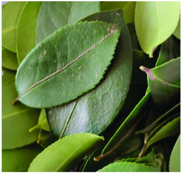
Fig. 1. Lossless, regular-shaped blade
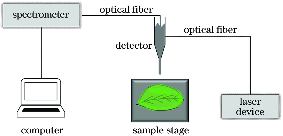
Fig. 2. Capture schematic of chlorophyll fluorescence spectrum
Fig. 3. Original full spectrum image
Fig. 4. Fluorescence spectrum pretreatment and model comparison process
Fig. 5. Fluorescence spectra of fresh tea leaves after smoothing treatment
Fig. 6. Variable stability results of UVE method screening
Fig. 7. Results of variable selection using UVE method
Fig. 8. Results of variable selection using SPA algorithm. (a) Relationship between number of selected variables and RMSEP; (b) locations of selected variables in processed spectra
Fig. 9. Prediction results of simplified PLS model
|
Table 1. Statistics on chlorophyll content
| ||||||||||||||||||||||
Table 2. PLS values before and after chlorophyll relative content treatment
|
Table 3. Descriptive statistics for calibration set and prediction set
| ||||||||||||||||||||||||||||||||||||||||
Table 4. Descriptive statistics of calibration set and prediction set
|
Table 5. Results of selecting optimal intervals step by step

Set citation alerts for the article
Please enter your email address
© Copyright 2018-2021 | Chinese Laser Press. All Rights Reserved 沪ICP备15018463号-20