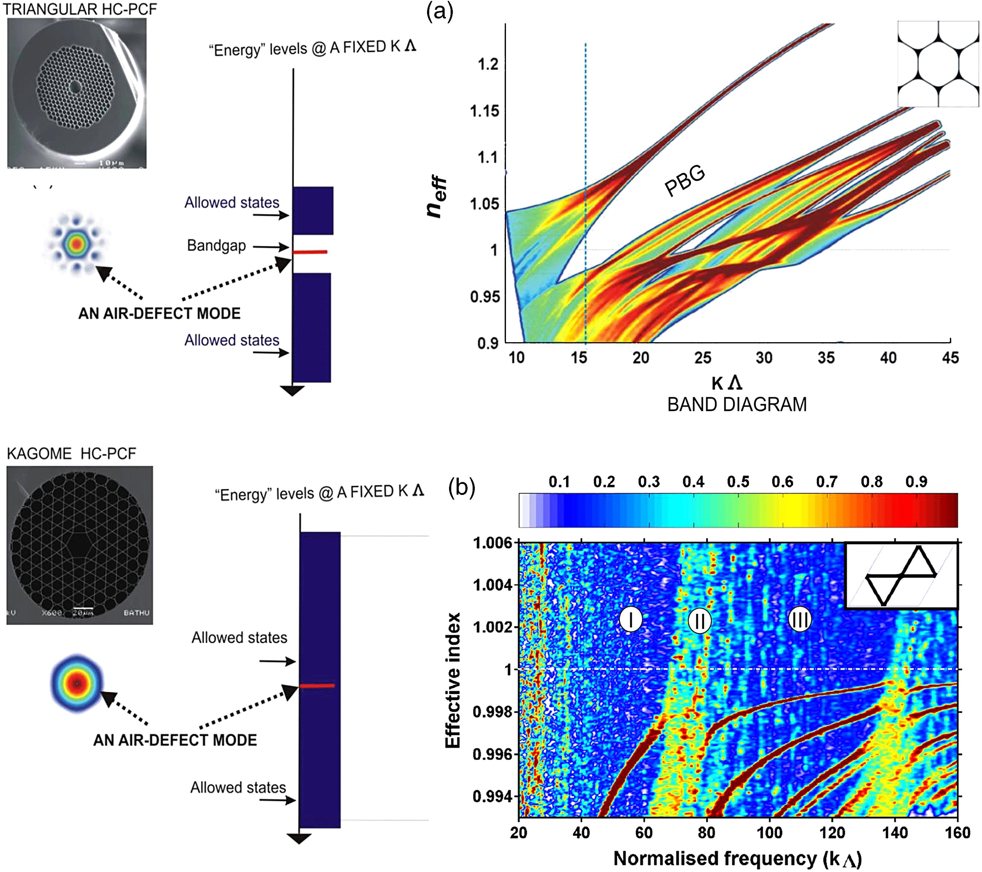
Fig. 1. (a) Top left: scanning electron micrograph of a triangular HC-PCF. Bottom left: near-field profile of the fundamental ( like) air guided core mode lying within a bandgap (Centre). Right: band diagram showing the presence of the PBG. (b) Same as (a) but for Kagome-lattice HC-PCF. The fundamental mode lies within a continuum of cladding modes and the band diagram does not exhibit a PBG.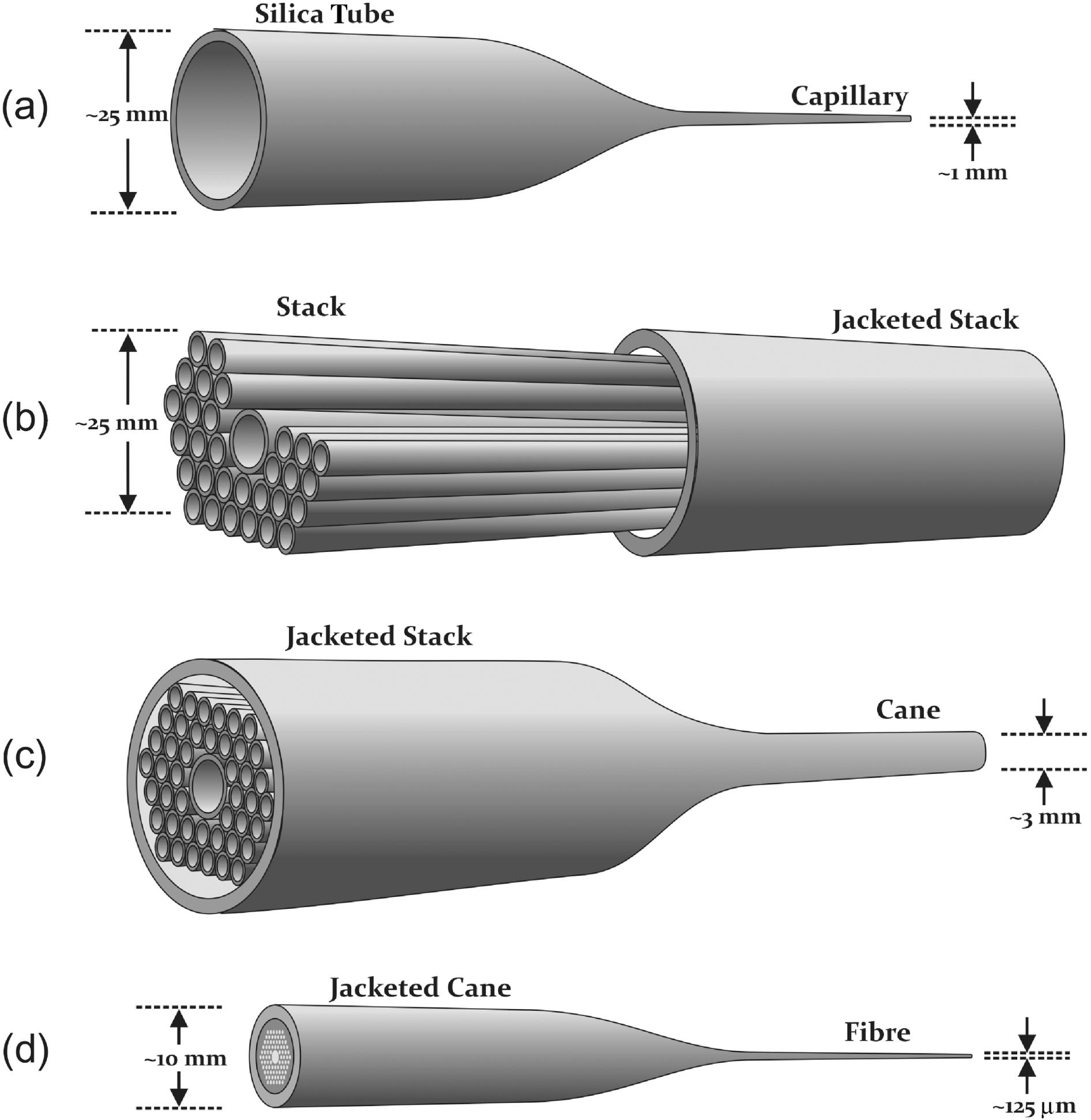

Fig. 2. An overview of the entire stack-and-draw technique: (a) drawing of capillaries; (b) capillaries are stacked and inserted into a larger tube; (c) the jacketed stack is drawn to smaller canes; and (d) the jacketed canes is drawn into fibre.

Fig. 3. (a) SEM image of the fabricated double-bandgap HC-PCF. (b) Near-field mode in the guided band. (c) Attenuation spectrum of the fibre showing two bandgaps. (d) Measured group delay (squares), and dispersion (solid lines) calculated based on a fourth-order polynomial fit to group delay data (dashed lines) at the second bandgap and the first bandgap^[23].

Fig. 4. (a) SEM image of the fabricated one-cell Kagome HC-PCF. (b) Near-field mode in the guided band. (c) Transmission spectrum of the fibre showing broad band guidance. (d) Measured group delay (red dots), and dispersion (black dotted line) calculated based on fourth-order polynomial fit to group delay data^[24].

Fig. 5. SEM image of the fabricated seven-cell three-ring hypocycloid-core Kagome fibre showing (a) the whole structure; (b) the 66– core^[32].

Fig. 6. (a) The fibre optical transmission spectra measured by the white-light source for 55 m (solid curve) and 5 m (dotted curve). (b) The fibre optical attenuation spectrum (solid black curve) and GVD (dashed red line). The dotted horizontal line shows the baseline of the attenuation figure. (c) Calculated near-field (NF) pattern with an MFD of . (d) Calculated intensity profile showing along the axis shown in the top-left inset. (e) Measured NF pattern showing an MFD of . (f) Measured far-field (FF) pattern^[32].

Fig. 7. Experimental set-up for the laser-induced spark-ignition experiment. : half wave plate  nm, G.P.: Glan polarizer, M: mirrors, L: lenses^[46].

Fig. 8. Air-breakdown demonstration (power density at the focal point approaching ) at the fibre output after focusing. At the bottom, the pictures show the spark ignition induced^[46].

Fig. 9. Output energy versus input energy for (a) a one-cell Kagome fibre with a silica core-surround thickness of 640 nm and (b) a seven-cell hypocycloid-core Kagome fibre with a silica core-surround thickness of 320 nm. The coupling efficiency and the damage threshold are indicated on the graphs; inserted in (a) and (b) are near-field intensity patterns recorded at the fibre output^[46].

Fig. 10. Set-up of the pulse-spread free experiment. HWP: half wave plate; PBS: polarizing beam splitter, OSA: optical spectrum analyser; AC: second harmonic intensity autocorrelator^[32].

Fig. 11. Spectral and temporal profiles of the deliver pulse trains when the fibre is filled with helium. (a) Optical spectra of the fibre input pulses with energy of (grey dashed curve) and output pulses with energies of (red), (pink), (orange), (yellow), (green), (cyan), (blue) and (purple). (b) intensity autocorrelation traces of fibre input pulses with energy of (grey dashed curve) and output pulses with energies of (orange), (yellow), (green), (cyan), (blue)^[32].

Fig. 12. Spectral and temporal profiles of the compressed pulse trains when the fibre is in ambient air. (a) Optical spectra of the fibre input pulses with energy of (grey dashed curve) and output compressed pulses with energies of (red), (pink), (orange), (yellow), (green), (cyan), (blue) and (purple). (b) Intensity autocorrelation traces of fibre input pulses with energy of (grey dashed curve) and output compressed pulses with energies of (red), (pink), (orange), (green), (cyan), (blue) and (purple). Note that the AC signal intensity is in arbitrary units and does not correspond to the power level^[32].

Fig. 13. FWHM pulse durations of the output pulses as a function of output pulse energies. Solid black square: fibre in helium. The blue line is a linear fit. Open black square: fibre in air. The vertical line shows the error bar. The red curve is an exponential fit^[32].

Table 1. Comparison of single-bandgap HC-PCF, double-bandgap HC-PCF, conventional circle-core or polygon-core Kagome HC-PCF and hypocycloid-core Kagome HC-PCF in terms of their guidance mechanism, dimension, optical attenuation, mode profile, mode overlap with silica, optical bandwidth and dispersion.