• Photonics Research
  • Vol. 12, Issue 3, 543 (2024)
Xiao Hu1、2, Tupei Chen2, Seongwoo Yoo2, and Dingyuan Tang1、*
Author Affiliations
  • 1Julong College, Shenzhen Technology University, Shenzhen 518118, China
  • 2School of Electrical and Electronic Engineering, Nanyang Technological University, Singapore 639798, Singapore
  • show less
    DOI: 10.1364/PRJ.508144 Cite this Article Set citation alerts
    Xiao Hu, Tupei Chen, Seongwoo Yoo, Dingyuan Tang. Cnoidal waves and their soliton limits in single mode fiber lasers[J]. Photonics Research, 2024, 12(3): 543 Copy Citation Text show less
    Evolution of an NLSE cnoidal wave in a ring fiber cavity. Color gradient indicates the increase of cavity nonlinearity. (a) A cnoidal wave at low cavity nonlinearity. (b) A cnoidal wave at the soliton limit. (c) Particle-like freely running solitons.
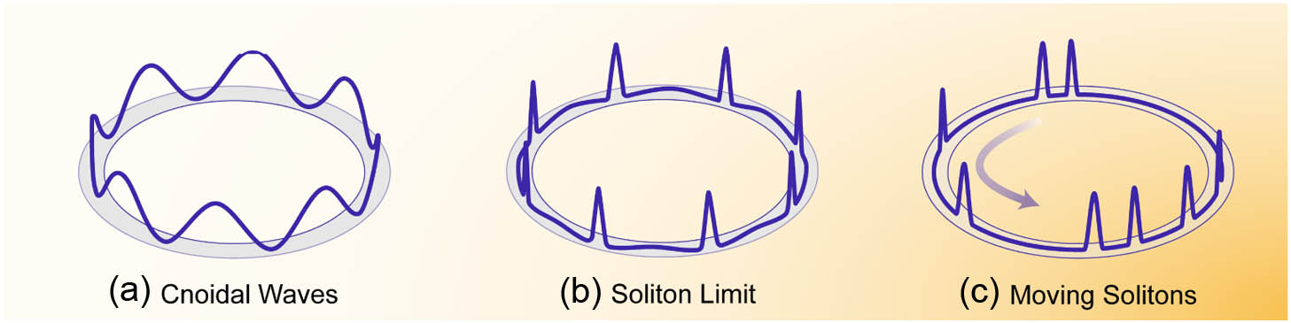
    Fig. 1. Evolution of an NLSE cnoidal wave in a ring fiber cavity. Color gradient indicates the increase of cavity nonlinearity. (a) A cnoidal wave at low cavity nonlinearity. (b) A cnoidal wave at the soliton limit. (c) Particle-like freely running solitons.
    Schematic of the experimental setup. The pump source is a 1480 nm Raman fiber laser. It has a maximum output power of 5 W. EDF, erbium-doped fiber (OFS-EDF80) with a group velocity dispersion (GVD) coefficient of β2=61.87 ps2/km; DCF, dispersion compensation fiber with a group velocity dispersion coefficient of β2=5.1 ps2/km; SMF, single mode fiber (SMF-28) with a group velocity dispersion coefficient of β2=−21.94 ps2/km; PI-ISO, polarization independent isolator; WDM, wavelength division multiplexer; OC, output coupler; BS, beam splitter; PD, photodetector; PC, polarization controller; OSC, oscilloscope; OSA, optical spectrum analyzer.
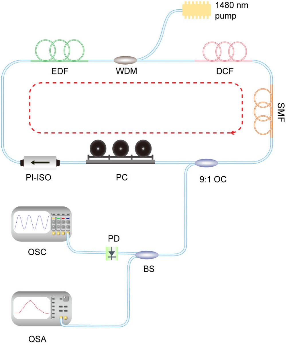
    Fig. 2. Schematic of the experimental setup. The pump source is a 1480 nm Raman fiber laser. It has a maximum output power of 5 W. EDF, erbium-doped fiber (OFS-EDF80) with a group velocity dispersion (GVD) coefficient of β2=61.87  ps2/km; DCF, dispersion compensation fiber with a group velocity dispersion coefficient of β2=5.1  ps2/km; SMF, single mode fiber (SMF-28) with a group velocity dispersion coefficient of β2=21.94  ps2/km; PI-ISO, polarization independent isolator; WDM, wavelength division multiplexer; OC, output coupler; BS, beam splitter; PD, photodetector; PC, polarization controller; OSC, oscilloscope; OSA, optical spectrum analyzer.
    Experimental results on formation of cnoidal waves with different periods in net anomalous dispersion regime. (a1) Oscilloscope trace of a cnoidal wave with period T=50 ps. (a2) Corresponding optical spectrum for (a1). (b1) Oscilloscope trace of a cnoidal wave with period T=33 ps. (b2) Corresponding optical spectrum for (b1). (c) Oscilloscope trace of a cnoidal wave with period T=4 ns.
    Fig. 3. Experimental results on formation of cnoidal waves with different periods in net anomalous dispersion regime. (a1) Oscilloscope trace of a cnoidal wave with period T=50  ps. (a2) Corresponding optical spectrum for (a1). (b1) Oscilloscope trace of a cnoidal wave with period T=33  ps. (b2) Corresponding optical spectrum for (b1). (c) Oscilloscope trace of a cnoidal wave with period T=4  ns.
    Experimental results on evolution of the cnoidal wave with period T=50 ps over 20 cavity roundtrips.
    Fig. 4. Experimental results on evolution of the cnoidal wave with period T=50  ps over 20 cavity roundtrips.
    Experimental results on soliton limit of cnoidal waves in net anomalous cavity dispersion regime. (a) Evolution of a periodic pulse train with period T=50 ps measured at t=0 s. (b) Evolution of the same periodic pulse train measured at t=120 s. (c) A train of bright pulses with a typical pulse width around several picoseconds. (d) The corresponding optical spectrum of (c).
    Fig. 5. Experimental results on soliton limit of cnoidal waves in net anomalous cavity dispersion regime. (a) Evolution of a periodic pulse train with period T=50  ps measured at t=0  s. (b) Evolution of the same periodic pulse train measured at t=120  s. (c) A train of bright pulses with a typical pulse width around several picoseconds. (d) The corresponding optical spectrum of (c).
    Simulation results on formation of cnoidal waves with different period with net anomalous cavity dispersion. Parameters used in the simulation: A=0.01;β2u,ave=−6.1 ps2/km; g=g0/[1+∫(|u|2+|v|2)dt/Es]; g0=50 km−1;Es=1 pJ;γ=3 W−1 km−1. (a), (b) Stable formation of a cnoidal wave with period T=50 ps; (c), (d) stable formation of a cnoidal wave with period T=100 ps; (e), (f) stable formation of a cnoidal wave with period T=200 ps. (g) Simulated optical spectrum for the cnoidal wave shown in (a).
    Fig. 6. Simulation results on formation of cnoidal waves with different period with net anomalous cavity dispersion. Parameters used in the simulation: A=0.01;β2u,ave=6.1  ps2/km; g=g0/[1+(|u|2+|v|2)dt/Es]; g0=50  km1;Es=1  pJ;γ=3  W1km1. (a), (b) Stable formation of a cnoidal wave with period T=50  ps; (c), (d) stable formation of a cnoidal wave with period T=100  ps; (e), (f) stable formation of a cnoidal wave with period T=200  ps. (g) Simulated optical spectrum for the cnoidal wave shown in (a).
    Simulation result on a periodic bright pulse train formation. Except g0=80 km−1, the other parameters used are the same as those for Fig. 6(a).
    Fig. 7. Simulation result on a periodic bright pulse train formation. Except g0=80  km1, the other parameters used are the same as those for Fig. 6(a).
    Experimental results on a state with freely moving particle-like solitons. (a) Evolution of a soliton pattern measured at t=0 s. (b) Evolution of a soliton pattern in the same time window but measured at t=120 s. (c) The corresponding optical spectrum of (a).
    Fig. 8. Experimental results on a state with freely moving particle-like solitons. (a) Evolution of a soliton pattern measured at t=0  s. (b) Evolution of a soliton pattern in the same time window but measured at t=120  s. (c) The corresponding optical spectrum of (a).
    Typical optical spectrum of dual-wavelength emission.
    Fig. 9. Typical optical spectrum of dual-wavelength emission.
    Evolution of cnoidal waves in the case where the periodic boundary condition is redefined by the dual-wavelength domain walls. (a) Formation of a cnoidal wave within a wavelength domain. (b) Pulses on the right-hand side of the domain are shaped into solitons and run out of the domain. (c) Solitons fill up the whole laser cavity.
    Fig. 10. Evolution of cnoidal waves in the case where the periodic boundary condition is redefined by the dual-wavelength domain walls. (a) Formation of a cnoidal wave within a wavelength domain. (b) Pulses on the right-hand side of the domain are shaped into solitons and run out of the domain. (c) Solitons fill up the whole laser cavity.
    Evolution of cnoidal waves in the case where the periodic boundary condition is redefined by the dual-wavelength domain walls. (a) Formation of a cnoidal wave within a wavelength domain. (b) Pulses on the right-hand side of the domain are shaped into solitons and run out of the domain. (c) Solitons fill up the whole laser cavity.
    Fig. 11. Evolution of cnoidal waves in the case where the periodic boundary condition is redefined by the dual-wavelength domain walls. (a) Formation of a cnoidal wave within a wavelength domain. (b) Pulses on the right-hand side of the domain are shaped into solitons and run out of the domain. (c) Solitons fill up the whole laser cavity.
    Experimental results on formation of cnoidal waves with different periods in net normal dispersion regime. (a) Oscilloscope trace of a cnoidal wave with period T=2.5 ns. (b) The corresponding optical spectrum of (a). (c) Oscilloscope trace of a cnoidal wave with period T=4 ns. (d) The corresponding optical spectrum of (c).
    Fig. 12. Experimental results on formation of cnoidal waves with different periods in net normal dispersion regime. (a) Oscilloscope trace of a cnoidal wave with period T=2.5  ns. (b) The corresponding optical spectrum of (a). (c) Oscilloscope trace of a cnoidal wave with period T=4  ns. (d) The corresponding optical spectrum of (c).
    Experimental results on the soliton limit of cnoidal waves in the net normal cavity dispersion regime. (a) A train of periodic dark pulses with a typical pulse width around hundreds of picoseconds. (b) The corresponding optical spectrum of (a).
    Fig. 13. Experimental results on the soliton limit of cnoidal waves in the net normal cavity dispersion regime. (a) A train of periodic dark pulses with a typical pulse width around hundreds of picoseconds. (b) The corresponding optical spectrum of (a).
    Simulation results on the formation of cnoidal waves in the net normal cavity dispersion regime. Parameters used in the simulations: A=0.01;β2u,ave=5.1 ps2/km; g=g0/[1+∫(|u|2+|v|2)dt/Es];Es=1 pJ;γ=3 W−1 km−1. (a) Evolution of a cnoidal wave with period T=1 ns and T=1 ns and g0=50 km−1. (b) A cnoidal wave pattern observed at the last cavity round trip of 10,000 in (a). (c) Evolution of a cnoidal wave to a train of dark pulses, T=1 ns and g0=100 km−1. (d) Dark pulse pattern observed at the last cavity round trip of 10,000 in (c). (e) Simulated optical spectrum for the cnoidal wave state shown in (a).
    Fig. 14. Simulation results on the formation of cnoidal waves in the net normal cavity dispersion regime. Parameters used in the simulations: A=0.01;β2u,ave=5.1  ps2/km; g=g0/[1+(|u|2+|v|2)dt/Es];Es=1  pJ;γ=3  W1km1. (a) Evolution of a cnoidal wave with period T=1  ns and T=1  ns and g0=50  km1. (b) A cnoidal wave pattern observed at the last cavity round trip of 10,000 in (a). (c) Evolution of a cnoidal wave to a train of dark pulses, T=1  ns and g0=100  km1. (d) Dark pulse pattern observed at the last cavity round trip of 10,000 in (c). (e) Simulated optical spectrum for the cnoidal wave state shown in (a).
    Xiao Hu, Tupei Chen, Seongwoo Yoo, Dingyuan Tang. Cnoidal waves and their soliton limits in single mode fiber lasers[J]. Photonics Research, 2024, 12(3): 543
    Download Citation